Week 8 - Simulating Cyclone separator with Discrete Phase Modelling

CHALLENGE - 8: Simulating Cyclone Separator with Discrete Phase Modelling

AIM:

To simulate the given cyclone separator geometry by using ANSYS FLUENT and calculate the separation efficiency and pressure drop.

OBJECTIVE:

1. To perform an analysis on a given cyclone separator model by varying the particle diameter from 1 μm to 5 μm and calculate the separation efficiency in each case.
2. To perform an analysis on a given cyclone separator model by varying the particle velocity from 1 m/sec to 5 m/sec and calculate the separation efficiency and pressure drop in each case.
3. To study different empirical models that used to calculate the cyclone separator efficiency.

THEORY:

Cyclonic separation is a method of removing particulates from an air, gas or liquid stream, without the use of filters, through vortex separation. Rotational effects and gravity are used to separate mixtures of solids and fluids. The method can also be used to separate fine droplets of liquid from a gaseous stream. The device which is used to perform the above principle is called cyclone separator.

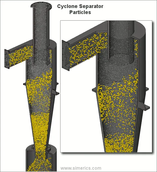Source: http://www.simerics.com/animation/cyclone_ani.gif

Formulae:

Pressure drop:

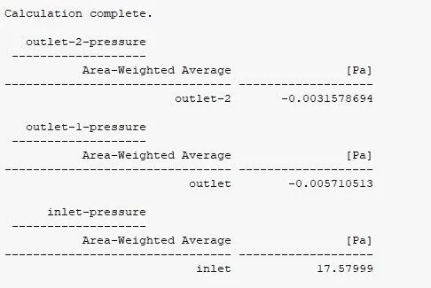
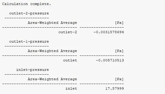
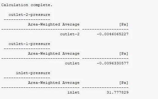
`DeltaP = "Inlet Pressure"-"Outlet-1 Pressure"`

Where Outlet-1 is the outlet at top (escape).

Separation efficiency:

`underset(s)(eta) = "No. of Particle Trapped"/"No. of Particle Tracked"`

Four empirical models used for cyclone separator efficiency

Iozia and Leith logistic model is a modified version of Barth Model, which is developed based on force balance. The model assumes that a particle carried by the vortex endures the influence of two forces: a centrifugal force, Z and a flow resistance, W. The collection efficiency of particle diameter dpi can be calculated from

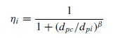
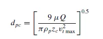
where `beta` is an expression for slope parameter and dpc is the 50% cut size given by Barth

,

LI and WANG model includes particle bounce or re-entrainment and turbulent diffusion at the cyclone wall. Li and Wang's model was developed based on the following assumptions:
1. The radial particle velocity and the radial concentration profile are not constant, for uncollected particles within the cyclones.
2. Boundary conditions with the consideration of turbulent diffusion coefficient and particle bounce re-entrainment on the cyclone wall.

KOCH and LICHT Model recognizes the inherently turbulent nature of cyclones and the distribution of gas residence times within the cyclone. It describes particle motion in the entry and the collection regions with some assumptions,
1. The tangential velocity of particles is equal to the tangential velocity of the gas flow i.e. 'no slip' in tangential direction between the particle and the gas.
2. The tangential velocity is related to the radius of the cyclone by UR^n = constant

LAPPLE model is a 1951 model developed by LAPPLE assuming that a particle entering a cyclone is evenly distributed along with the inlet opening. It is based on Force Balance without considering the flow resistance. In this model, the particle that travels from inlet half-width to the wall in the Cyclone is collected with 50% efficiency.

PROCEDURE:

1. Open ANSYS Workbench 2022R2 select Fluid Flow (Fluent) from Toolbox.

2. Rename the file and left click Geometry and select New Spaceclaim Geometry.

3. Open the geometry STEP or SLDPRT of the geometry in spaceclaim.

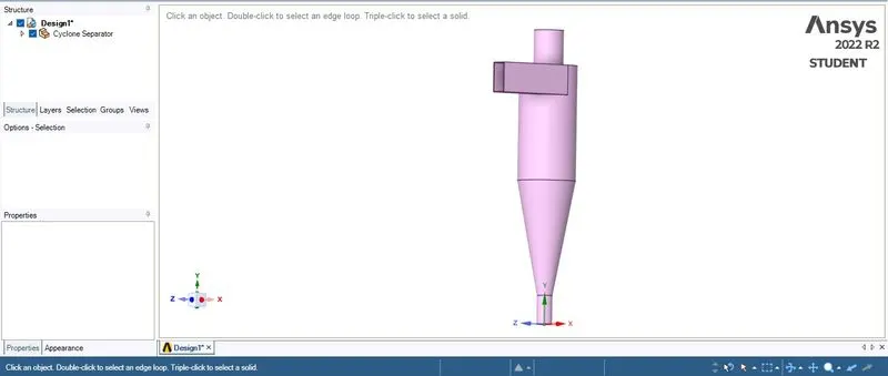
4. Extract the fluid volume by selecting Extract Volume option from Prepare menu on top bar. Then select the edges and click the tick mark now a new volume is created and which can be visible on tree. Now suppress the geometry by selecting the suppress from physics option which help to provide only the extracted volume for the analysis.

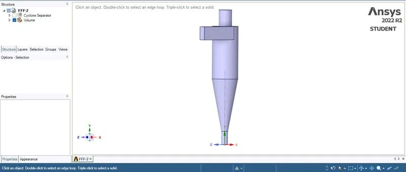
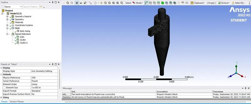
5. Close SpaceClaim and double click on Mesh. Meshing window will appear. Mark Inlet, Outlet and Outlet-2 on geometry by right clicking each part and selecting Create Name Selection. Now select the mesh from the tree and generate mesh with an appropriate element size (10 mm). The figure shown below represent the geometry after meshing.

6. Close Meshing and double click on Setup, select Double Precision and Fluent window will open. Check all the values and make necessary correction if needed.

7. Select appropriate conditions mentioned below.

Part - 1:- Velocity = 3m/s and diameter varies from 1 μm to 5 μm

Solver - Pressure Based

Viscous - k-epsilon model with RNG

Discrete Phase Model - on, Enable interaction with continuous phase and update DPM sources flow iteration

Provide Injection as Surface type and select Particle its velocity (3 m/s) and diameter (1 μm to 5 μm)

Materials - Fluid, Air

Inlet - Velocity Inlet, Velocity = 3m/s, DPM - Reflect

Outlet - Pressure Outlet, DPM - Escape

Outlet -2 - Pressure Outlet, DPM - Trap

Define surface report with area weighted average of pressure at inlet and both the outlets

Solution Initialization - Standard Initialization.

Part - 2:- Velocity = 1m/s to 5m/s and diameter = 5 μm

Solver - Pressure Based

Viscous - k-epsilon model with RNG

Discrete Phase Model - on, Enable interaction with continuous phase and update DPM sources flow iteration

Provide Injection as Surface type and select Particle its velocity (1m/s to 5m/s) and diameter (5 μm)

Materials - Fluid, Air

Inlet - Velocity Inlet, Velocity = 1m/s to 5m/s , DPM - Reflect

Outlet - Pressure Outlet, DPM - Escape

Outlet -2 - Pressure Outlet, DPM - Trap

Define surface report with area weighted average of pressure at inlet and both the outlets

Solution Initialization - Standard Initialization.

8. After assigning all the factors click on Run Calculation and set number of iteration and calculate.

9. After completing the calculation export Particle History Data by selecting the injection type and folder to write the data.

10. Now close ANSYS FLUENT and open CFD post and import the Particle History Data and plot the contours.

The results obtained are discussed in the next session.

RESULTS AND DISCUSSION:

Part - 1:- Velocity = 3m/s and diameter varies from 1 μm to 5 μm

Case - 1: Diameter - 1 μm

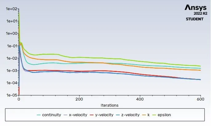
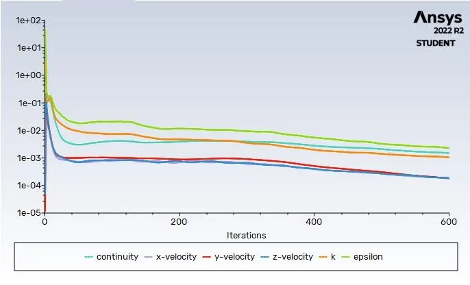
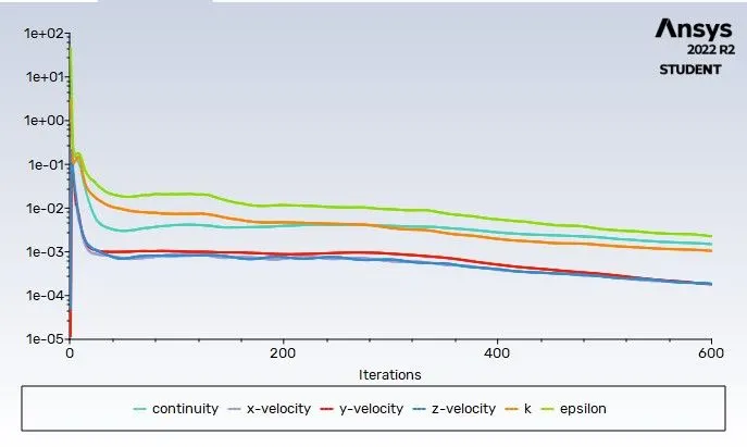
a. Residual Plot

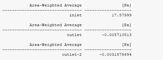
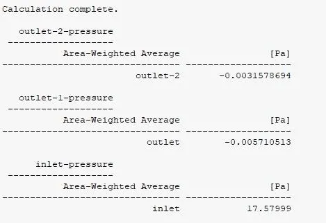
b. Calculated Pressure and Particle History

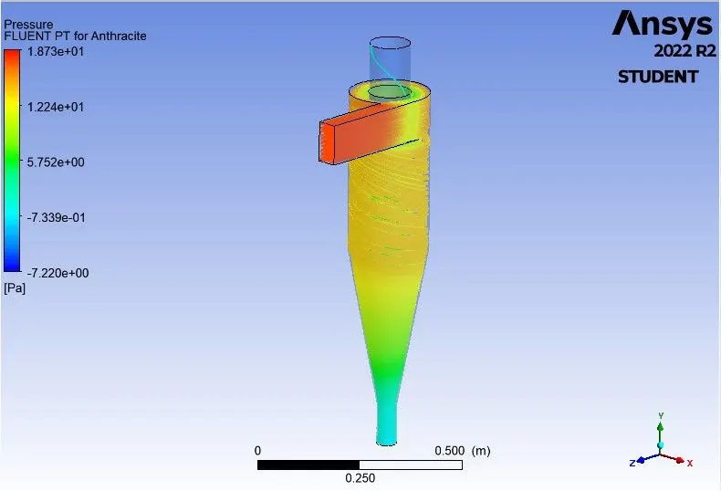
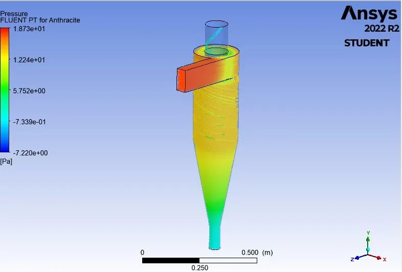
c. Pressure Contour

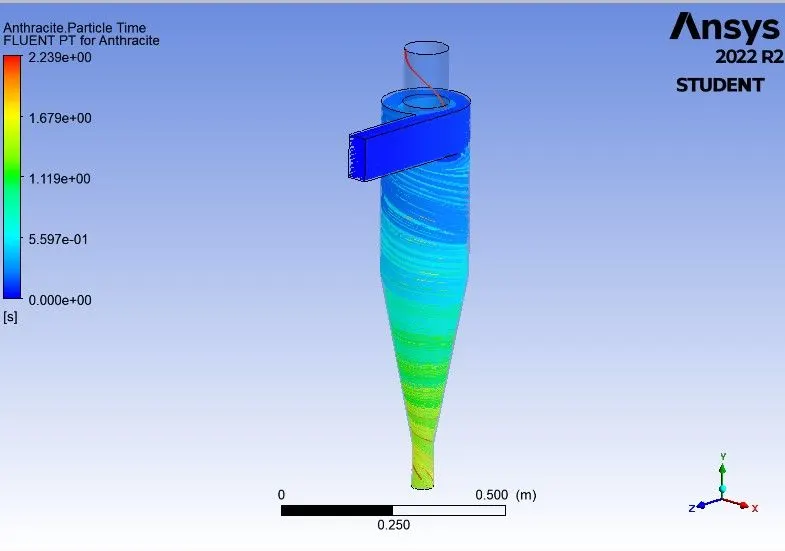
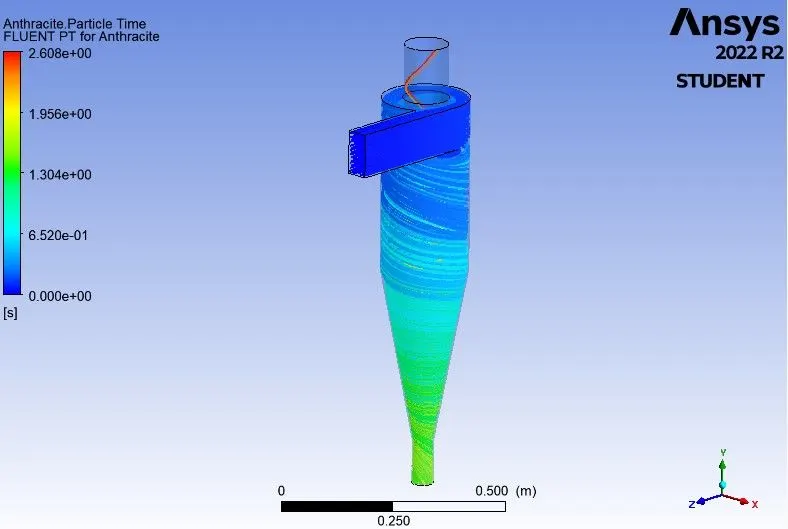
d. Anthracite Particle Time Contour

Case - 2: Diameter - 2μm

a. Residual Plot

b. Calculated Pressure and Particle History

c. Pressure Contour

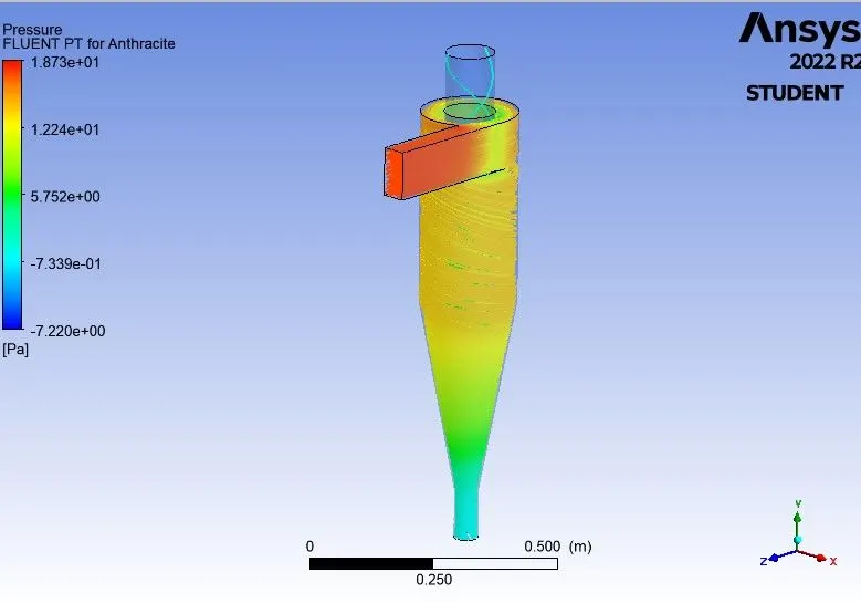
d. Anthracite Particle Time Contour

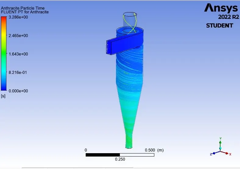
Case - 3: Diameter - 3 μm

a. Residual Plot

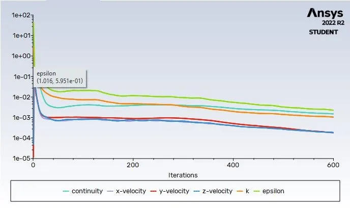
b. Calculated Pressure and Particle History

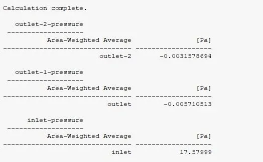
c. Pressure Contour

d. Anthracite Particle Time Contour

Case - 4: Diameter - 4μm

a. Residual Plot

b. Calculated Pressure and Particle History

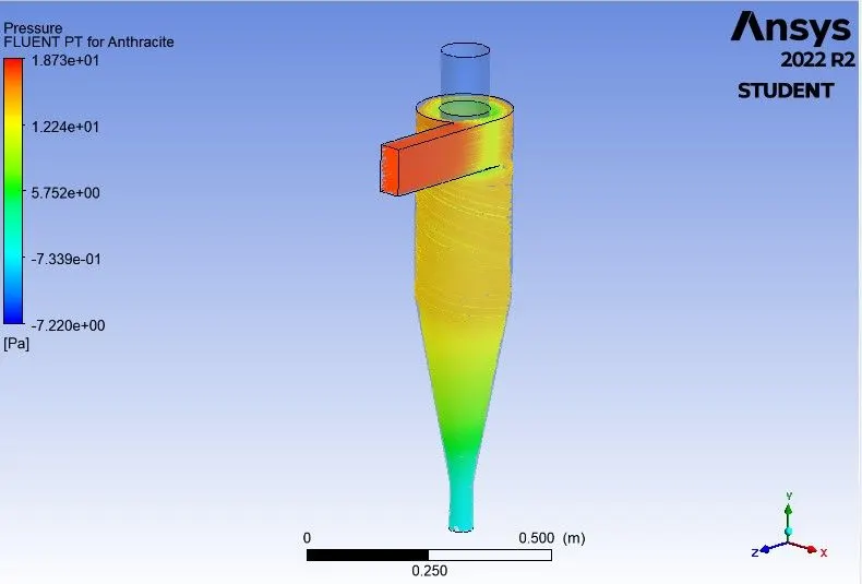
c. Pressure Contour

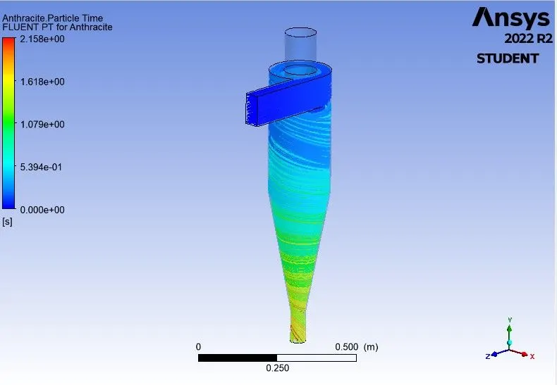
d. Anthracite Particle Time Contour

Case - 5: Diameter - 5μm

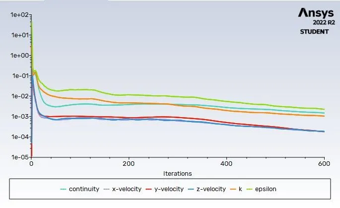
a. Residual Plot

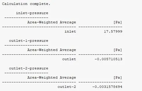
b. Calculated Pressure and Particle History

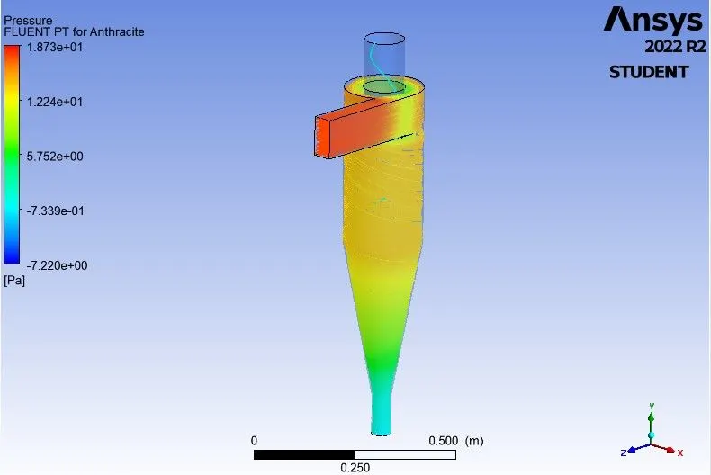
c. Pressure Contour

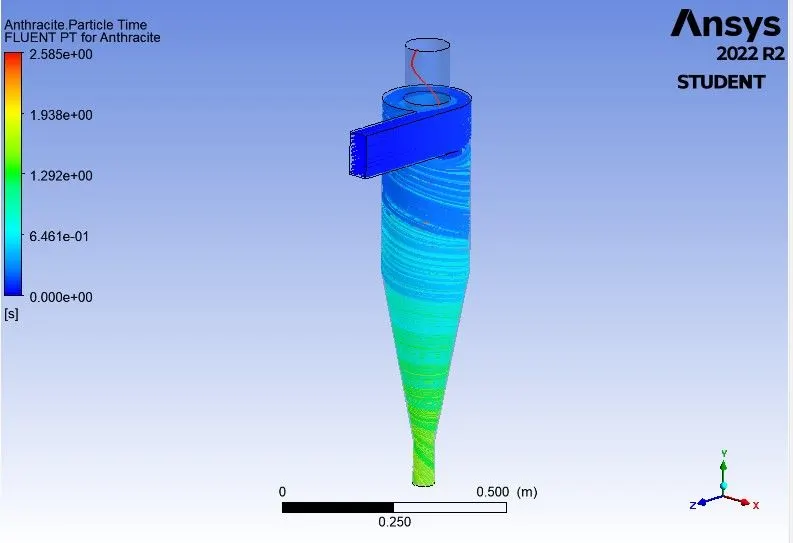
d. Anthracite Particle Time Contour

	Particle Tracked	Particle Escaped	Particle Trapped	Separation Efficiency	Pressure Drop
Case - 1	124	1	123	99.19%	17.576Pa
Case - 2	124	2	122	98.38%	17.576Pa
Case - 3	124	2	122	98.38%	17.576Pa
Case - 4	124	0	124	100%	17.576Pa
Case - 5	124	1	123	99.19%	17.576Pa

Part - 2:- Velocity = 1m/s to 5m/s and diameter = 5 μm

Case - 1: Velocity = 1m/s

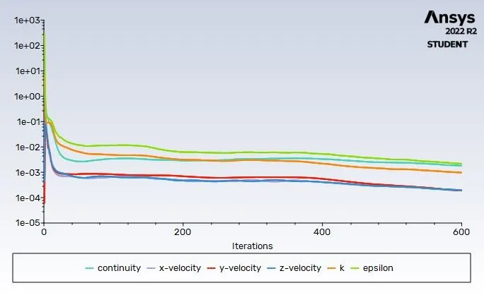
a. Residual Plot

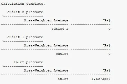
b. Calculated Pressure and Particle History

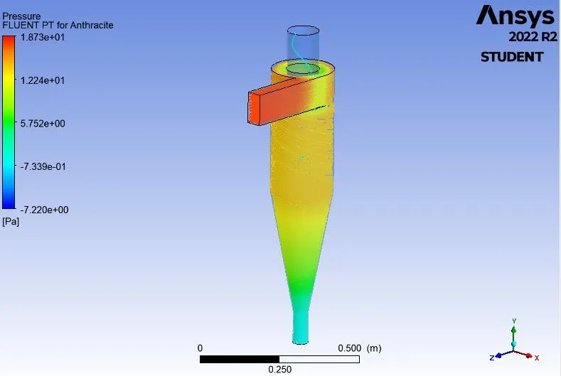
c. Pressure Contour

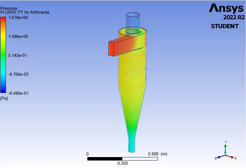
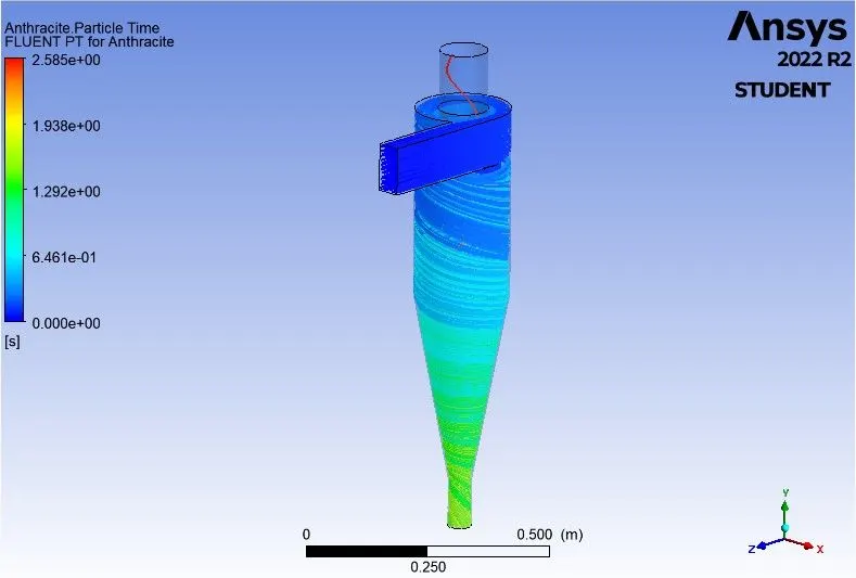
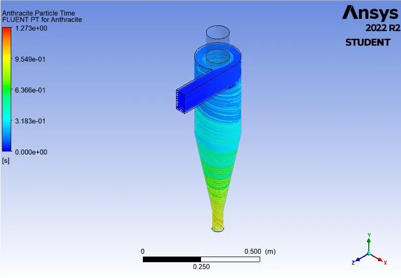
d. Anthracite Particle Time Contour

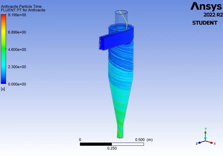
Case - 2: Velocity = 2m/s

a. Residual Plot

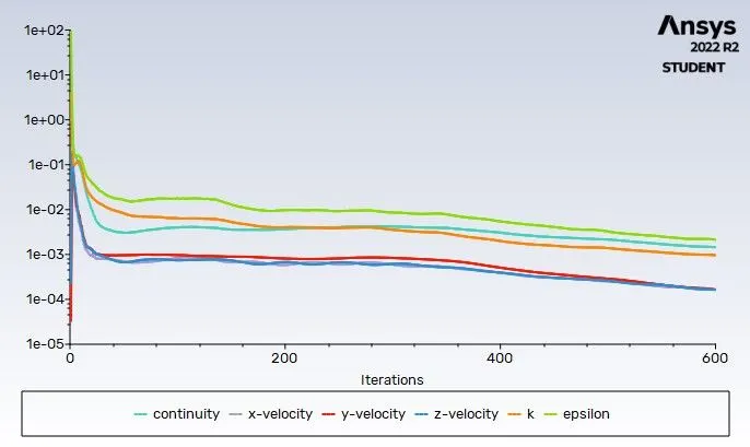
b. Calculated Pressure and Particle History

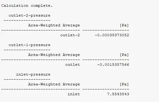
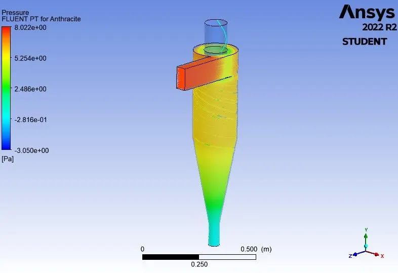
c. Pressure Contour

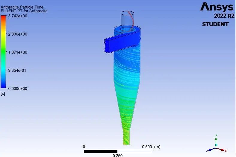
d. Anthracite Particle Time Contour

Case - 3: Velocity = 3m/s

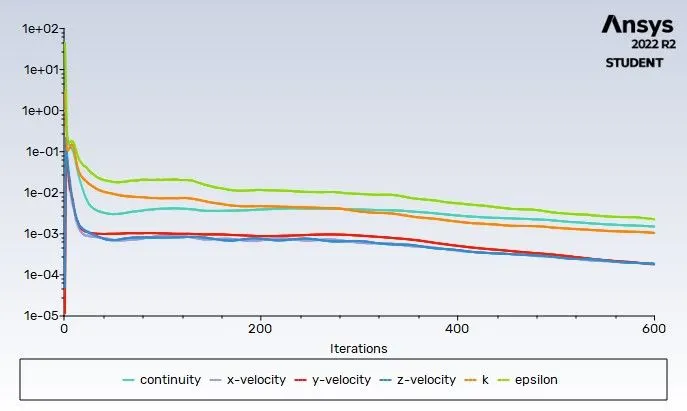
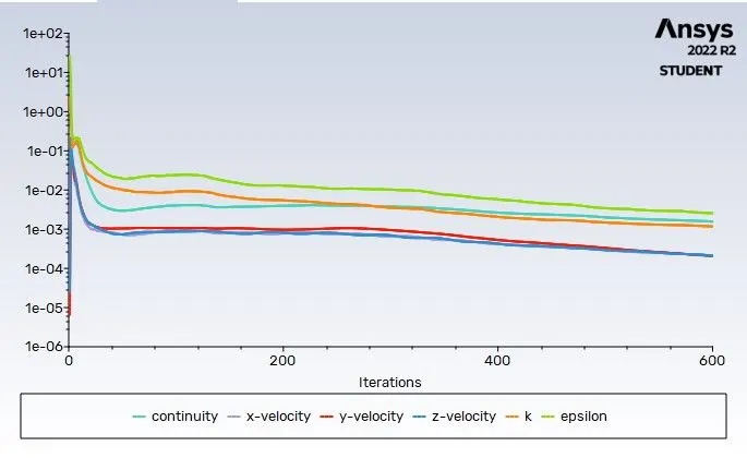
a. Residual Plot

b. Calculated Pressure and Particle History

c. Pressure Contour

d. Anthracite Particle Time Contour

Case - 4: Velocity = 4m/s

a. Residual Plot

b. Calculated Pressure and Particle History

c. Pressure Contour

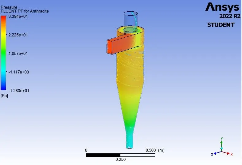
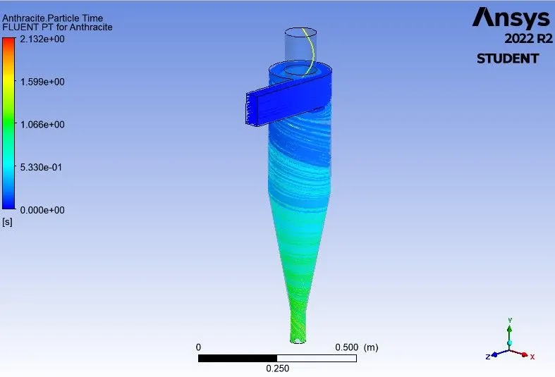
d. Anthracite Particle Time Contour

Case - 5: Velocity = 5m/s

a. Residual Plot

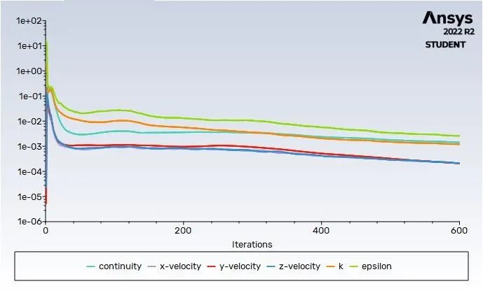
b. Calculated Pressure and Particle History

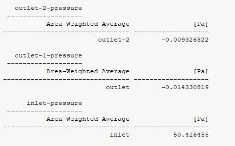
c. Pressure Contour

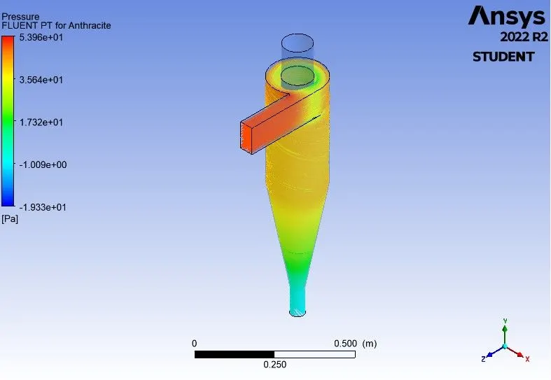
d. Anthracite Particle Time Contour

	Particle Tracked	Particle Escaped	Particle Trapped	Separation Efficiency	Pressure Drop
Case - 1	124	1	123	99.19%	1.607 Pa
Case - 2	124	1	123	99.19%	7.5539 Pa
Case - 3	124	1	123	99.19%	17.5767 Pa
Case - 4	124	1	123	99.19%	31.7724 Pa
Case - 5	124	0	124	100%	50.4071 Pa

From the above two tables and contours it is observed that for Part-1 when the particle diameter increases pressure drop remains same, that is no effect in pressure drop with particle diameter. Similarly for Part-2 with increase in velocity separation efficiency almost remains same upto 4 cases but pressure drop increases with increase in velocity. The optimum condition for the Part-1 simulation is Case 3 (Dia = 4e-06, vel = 3m/s, Simulation efficiency = 100%). Similarly for Part-2 the optimum condition if there is pressure drop consideration is Case - 1 (Dia = 5e-06m, vel = 1m/s, Simulation efficiency = 99.19% and Pressure drop = 1.607 Pa) otherwise, Case -5 (Dia = 5e-06m, vel = 5m/s, Simulation efficiency = 100% and Pressure drop = 50.4071 Pa).

CONCLUSION:

Simulation of the given cyclone separator with different operating conditions have been carried out by using ANSYS FLUENT. From the simulation optimum condition is selected for obtaining maximum efficiency and minimal pressure drop. A study about cyclone separator and different empirical model for separation efficiency calculation is also done.