Week 8 - Simulating Cyclone separator with Discrete Phase Modelling

Simulating Cyclone separator with Discrete Phase Modelling

Aim:

To perform analysis on cyclone separator and calculate the separation efficiency and pressure drop.

Objective:

1. To write a few words about any four empirical models used to calculate the cyclone separator efficiency.
2. To perform an analysis on a given cyclone separator model by varying the particle diameter from 1 μm to 5 μm and calculating the separation efficiency in each case. Discuss the results. [Use both the velocity's as 3m/sec.]
3. To perform an analysis on a given cyclone separator model by varying the particle velocity from 1 m/sec to 5 m/sec and calculate the separation efficiency and pressure drop in each case. Discuss the results. [Use particle diameter size as 5 μm for all cases & keep flow velocity the same as particle velocity]

Introduction:

What is the Discrete Phase Model (DPM)?

Discrete Phase Model is a subsection to Multiphase flows. A discrete phase model (DPM) is used when the aim is to investigate the behavior of the particles from a Lagrangian view and a discrete perspective. The difference between the Lagrangian and the Eulerian view is that fluid behavior in the Lagrangian view is examined based on particle tracking of a particulate flow; Whereas fluid behavior is considered in the Eulerian view based on the assumption of a finite volume element in the fluid flow path.

In Discrete Phase Model, the continuous phase is solved using Navier-Stokes equations. At the same time, the discrete phase is simulated by tracking a large number of particles, bubbles, or droplets passing through the calculated continuous flow field. It should be noted that the discrete phase can exchange momentum, mass, and energy with the continuous phase. This method can be made much simpler by ignoring the interaction of particles (as well as droplets and bubbles) with each other. Of course, this can happen when the discrete phase, even with a large mass, has a much smaller volume (less than 10%) than the continuous phase. After each iteration of the continuous phase calculations, the particle paths (as well as bubbles or droplets) are calculated and determined separately. [1]

Types of cyclone separators:

Reverse flow: Reverse flow cyclone separators are cone-shaped. Gas enters the top of the separator body, flows downwards, then flows back upwards and is discharged.

Axial flow: For axial flow (a.k.a. straight through) cyclone separators, gas enters at one end and is discharged at the opposite end. Axial flow separators are not as common as reverse flow separators. [2]

Emperical models used to calculate cyclone separator efficiency:

• IOZIA AND LEITH MODEL

Iozia and Leith (1990) logistic model is a modified version of Barth (1956) model which is developed based on force balance. The model assumes that a particle carried by the vortex endures the influence of two forces: a centrifugal force, Z, and a flow resistance, W.

The collection efficiency ηi of particle diameter dpi can be calculated from `= η=1/(1+(d_pc/d_pi )^β )`

• LI AND WANG MODEL

The Li and Wang (1989) model include particle bounce or re-entrainment and turbulent diffusion at the cyclone wall. A two-dimensional analytical expression of particle distribution in the cyclone is obtained. Li and Wang model was developed based on the following assumptions:

1. The radial particle velocity and the radial concentration profile are not constant, for uncollected particles within the cyclones.
2. Boundary conditions with the consideration of turbulent diffusion coefficient and particle bounce re-entrainment on the cyclone wall.

The resultant expression of the collection efficiency for particles of my size is given as,

`η=1-exp⁡〖{-λθ}〗`

• KOCH AND LICHT MODEL

Koch and Licht (1977) collection theory recognized the inherently turbulent nature of cyclones and the distribution of gas residence times within the cyclone. Koch and Licht describe particle motion in the entry and collection regions with the additional following assumptions:

1. The tangential velocity of a particle is equal to the tangential velocity of the gas flow, i.e. there is no slip in the tangential direction between the particle and the gas.
2. The tangential velocity is related to the radius of the cyclone by: uRn = constant.

`η=1-{1-(12D)^((0.14) )/2.5} {(T+460)/530}^0.3`

• LAPPLE MODEL

Lapple (1951) model was developed based on force balance without considering the flow resistance. Lapple assumed that a particle entering the cyclone is evenly distributed across the inlet opening. The particle that travels from inlet half width to the wall in the cyclone is collected with 50% efficiency. The semi empirical relationship developed by Lapple (1951) to calculate a 50% cut diameter [3]

The efficiency of collection of any size of particle is given by,

`η=1/(1+(d_pc/d_pi )^2 )`

Approach and solving:

• By varying the particle diameter from 1 μm to 5 μm and calculate the separation efficiency in each case. [Velocity= 3m/s]
• By varying the particle velocity from 1 m/sec to 5 m/sec and calculate the separation efficiency and pressure drop in each case. [Diameter= 5 μm]

PROCEDURE:

• Geometry
• Mesh
• Setup
• Solution
• Results

Pre-Processing:

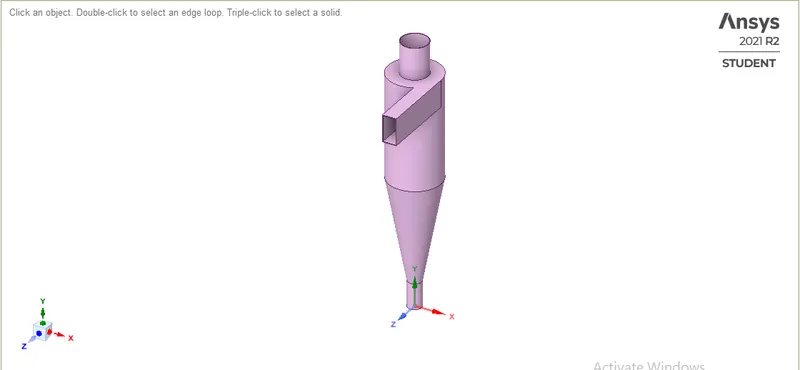
Geometry:

1. Import geometry to spaceclaim.
2. Interference check
3. Share topology
4. Extra-edges

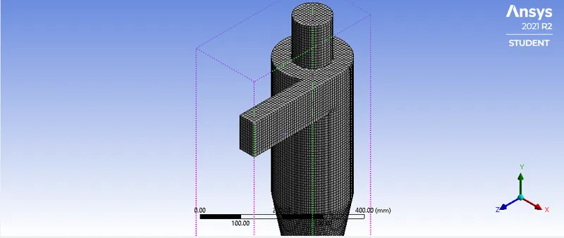
Meshing

Mesh size: 8mm

No of node: 59810

No of elements: 52613

Setup:

General: Pressure based, absolute, Steady state

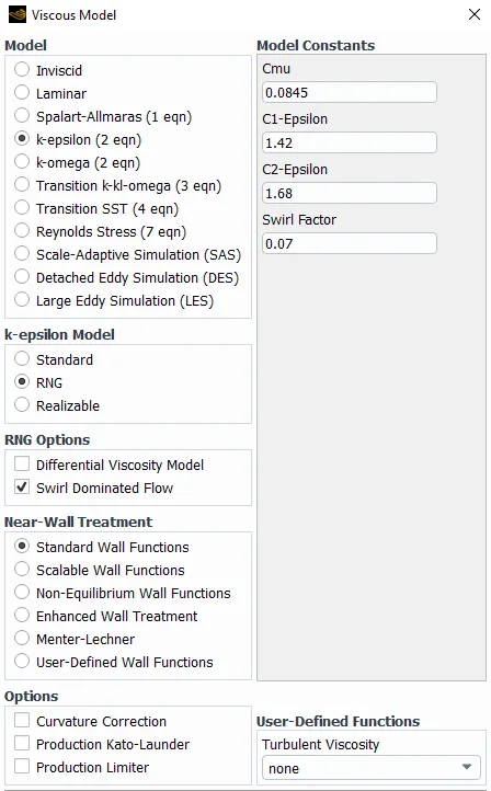
Model:

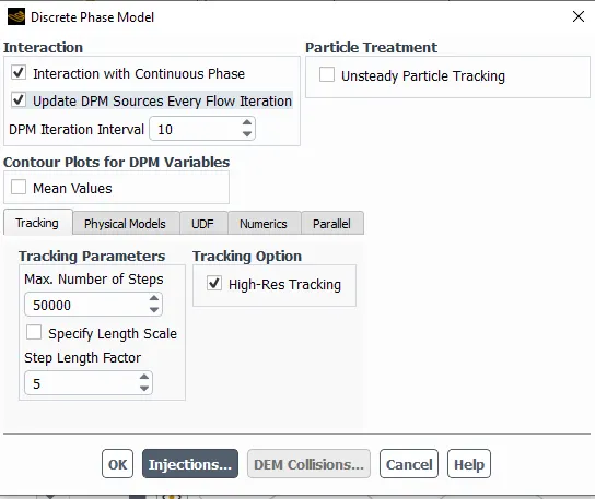
Discrete Phase Model:

Injection parameter:

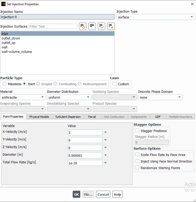
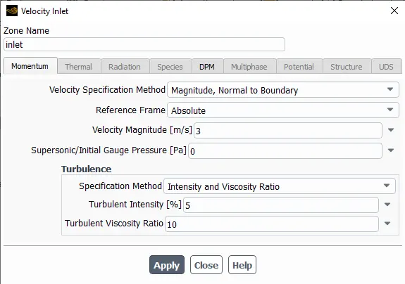
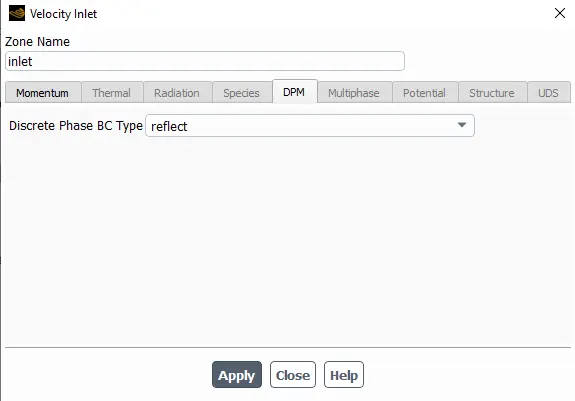
Inlet conditions:

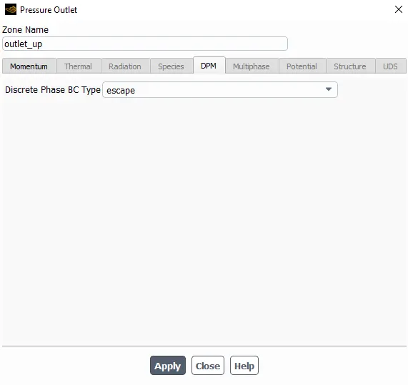
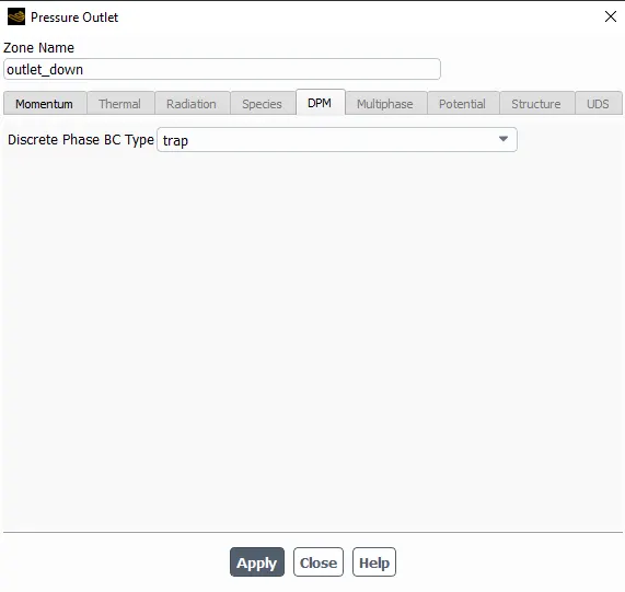
Outlet condition (up)

Outlet condition (down)

Results

Simulation 1

Case	Particle size (𝝁m)	Velocity (m/s)
1	1	3
2	3	3
3	5	3

Simulation 2

Case	Particle size (𝝁m)	Velocity (m/s)
1	5	1
2	5	3
3	5	5

Simulation 1

Case1

Particle size: 1𝝁m

Velocity: 3m/s

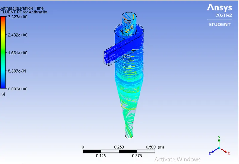
Number of tracked particles= 91, trapped particles= 45

Separation efficiency= No of particles trapped/ No of particles tracked

Separation efficiency= 45/91= 49.45%

Case2

Particle size: 3𝝁m

Velocity: 3m/s

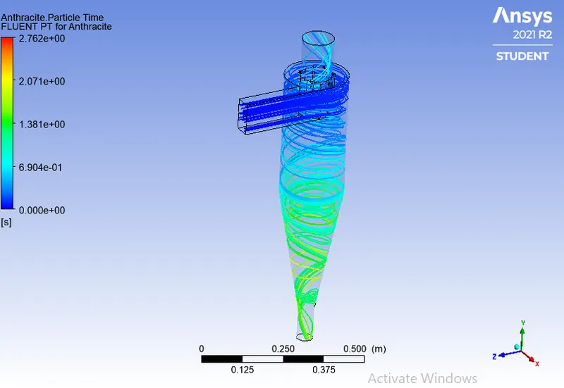
Number of tracked particles= 91, trapped particles= 55

Separation efficiency= No of particles trapped/ No of particles tracked

Separation efficiency= 55/91= 60.43%

Case3

Particle size: 5𝝁m

Velocity: 3m/s

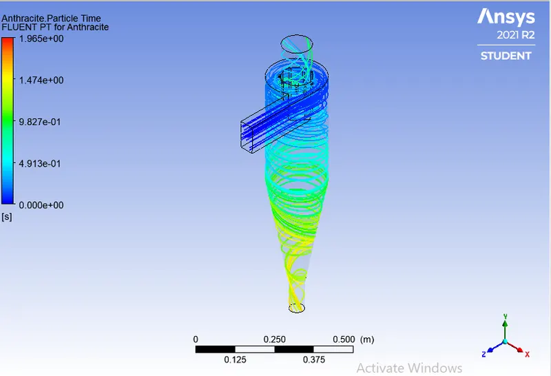
Number of tracked particles= 91, trapped particles= 59

Separation efficiency= No of particles trapped/ No of particles tracked

Separation efficiency= 59/91= 64.83%

Simulation2

Case1

Particle size: 5𝝁m

Velocity: 1m/s

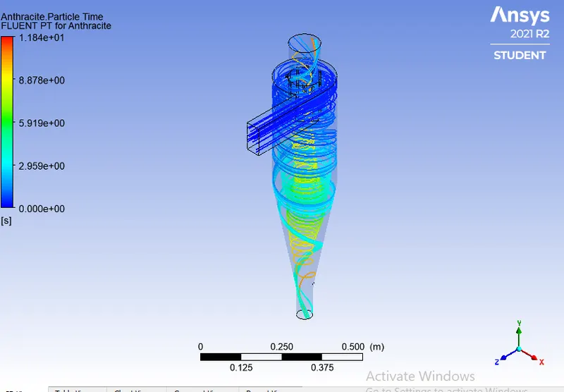
Number of tracked particles= 91, trapped particles= 53

Separation efficiency= No of particles trapped/ No of particles tracked

Separation efficiency= 53/91= 58.24%

Pressure drop= 1.7Pa

Case2

Particle size: 5𝝁m

Velocity: 3m/s

Number of tracked particles= 91, trapped particles= 59

Separation efficiency= No of particles trapped/ No of particles tracked

Separation efficiency= 59/91= 64.83%

Pressure drop= 17.28Pa

Case3

Particle size: 5𝝁m

Velocity: 5m/s

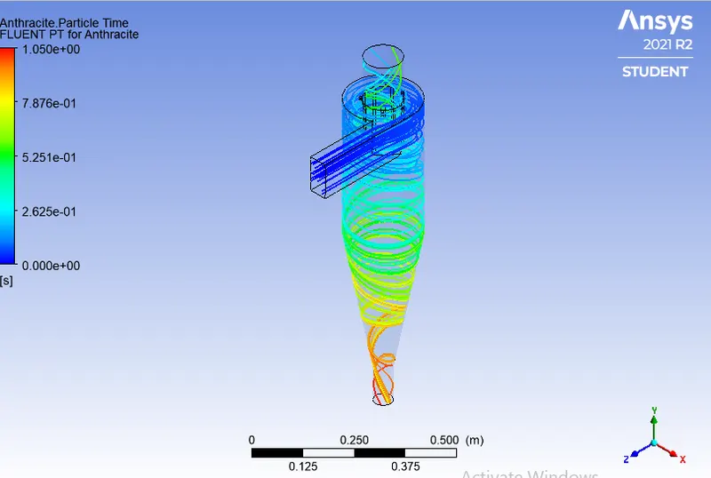
Number of tracked particles= 91, trapped particles= 60

Separation efficiency= No of particles trapped/ No of particles tracked

Separation efficiency= 60/91= 66%

Pressure drop= 49.81Pa

Conclusion:

• In simulation1, it was observed that the separator efficiency increases with an increase in particle diameter for constant velocity. So we can conclude that the cyclone separator can efficiently trap the larger particle but when it comes to particles with smaller diameter it is not that efficient. Hence the diameter of particles plays an important role in maintaining the efficiency of the cyclone separator.
• In simulation2, it was observed that the velocity also affects the efficiency of the separator. With an increase in inlet velocity, the efficiency of the separator was observed to be increased.

References:

[1] https://www.mr-cfd.com/services/fluent-modules/discrete-phase-model-dpm/?v=c86ee0d9d7ed

[2] https://savree.com/en/encyclopedia/cyclone-separator-working-principle-dust-separator

[3] http://dspace.unimap.edu.my/xmlui/bitstream/handle/123456789/13571/054-058_empirical%20models.pdf?sequence=1