Week 2 - Flow over a Cylinder.

Flow over cylinder

Aim:

PART -1

1. Simulate the flow with steady and unsteady cases and calculate the Strouhal Number for Re=100.

PART-2

1. Calculate the coefficient of lift and drag over a cylinder by setting the Reynolds number to 10,100,1000,10000,100000. (Run with steady solver).
2. Discuss the effect of Reynolds number on the coefficient of drag. (Error within 5%).

Introduction:

Karman Vortex Street:

Karman Vortex Street is a repeating pattern of swirling vortices, caused by the process of vortex shedding which is responsible for the unsteady separation of flow over a blunt body.

A vortex street will form only at a certain range of flow velocities, specified by a range of Reynolds numbers (Re), typically above a limiting Re value of about 90. [1]

Strouhal number:

Strouhal number is a dimensionless number describing oscillating flow mechanisms.

The parameter is named after Vincenc Strouhal, a Czech physicist who experimented in 1878 with wires experiencing vortex shedding and singing in the wind. The Strouhal number is an integral part of the fundamentals of fluid mechanics. [2]

Y Plus:

It's important that your mesh near the wall is properly sized to ensure accurate simulation of the flowfield. Hence Y helps in computing the height of the 1^st mesh cell of the wall for proper tracking of the boundary layer near the wall.

Formulation:

`St=fL/U`

Where,

`Where, St =` Strouhal number

`f` = Frequency of vortex shedding

`L`= Characteristic length

`U`= Flow velocity

`Re=(ρ*V*L)/μ`

Where,

`Re`= Reynolds number

`ρ`= density of the fluid

`V`= flow velocity

`L`= characteristic length

`μ`= dynamic viscosity

Solving and Modeling approach

Part-1:

As per the Karman Vortex Street,

Re= 100,

Density = 1 kg/,

Dynamic viscosity = 0.02 kg/m-s.

I performed the steady and unsteady simulation and calculated the shrouhal’s number.

Part-2

By using a steady solver,

For Re= 10,100,1000,10000,100000. I calculated the coefficient of drag and lift.

PROCEDURE:

Pre-Processing:

Geometry

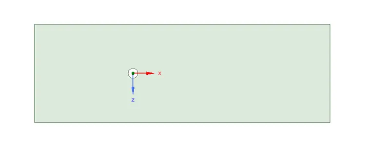
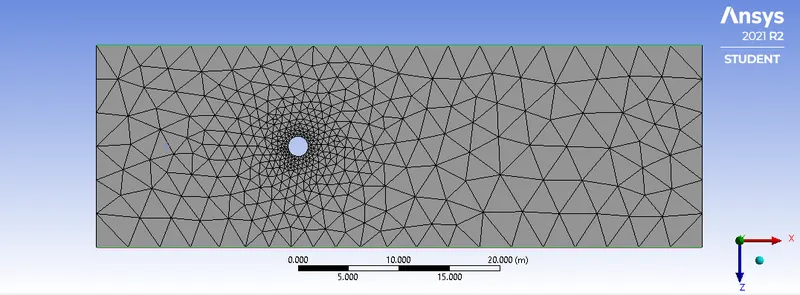
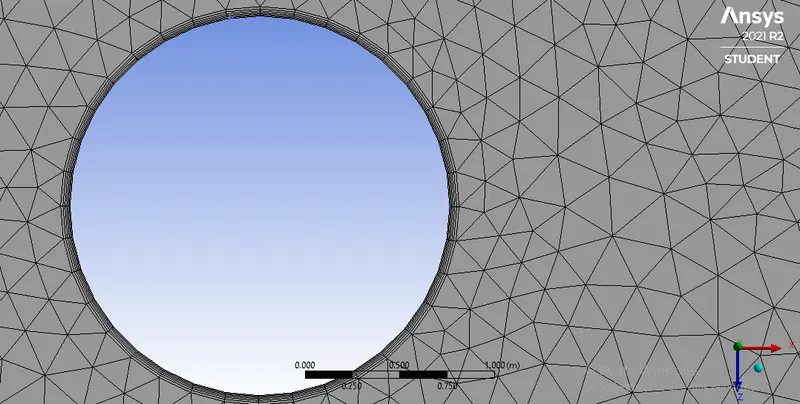
Mesh

Element size: 0.25m

No of nodes: 20697

Cell count: 40502

Triangular mesh

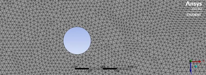
Fine meshing

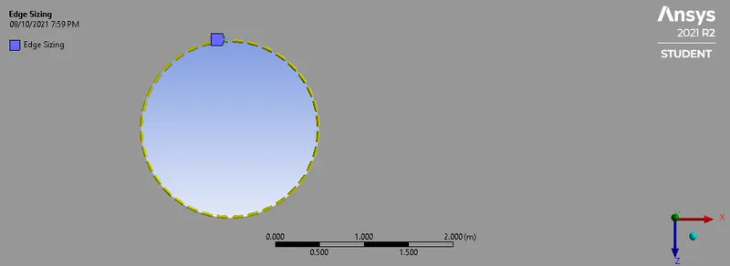
Edge smoothning: making the edges of the cylinder smooth, that is we are sizing the object

Mesh>Insert>Sizing>selecting the body> selecting the edge>Apply>type>no of divisions> 36

Inflation layers:

Inflation layer height: 5mm

Maximum layers: 6

Part-1

Re= 100,

Density = 1 kg/,

Dynamic viscosity = 0.02 kg/m-s.

Setup

Steady:

General: Pressure based, absolute, Steady state

Model: Viscous laminar

Material: User-defined

Density: 1 kg/

Viscosity: 0.02 kg/m-s

Cell zone: fff_volume (user material)

Boundary condition: inlet-velocity= 1m/s

Outlet = 0 Pa (1 atm)

Wall = no-slip condition

Method: Simple

Definitions: vertex average, lift, drag

Initialization: Hybrid initialization

Run-calculation: 800-iterations

Transient:

General: Pressure based, absolute, transient state

Model: Viscous laminar

Material: User-defined

Density: 1 kg/

Viscosity: 0.02 kg/ms

Cell zone: fff_volume (user material)

Boundary condition: inlet-velocity= 1m/s

Outlet = 0 Pa (1 atm)

Wall = no-slip condition

Method: Coupled

Definitions: vertex average, lift, drag

Initialization: Hybrid initialization

Run-calculation: 800-iterations

Results

Post-Processing

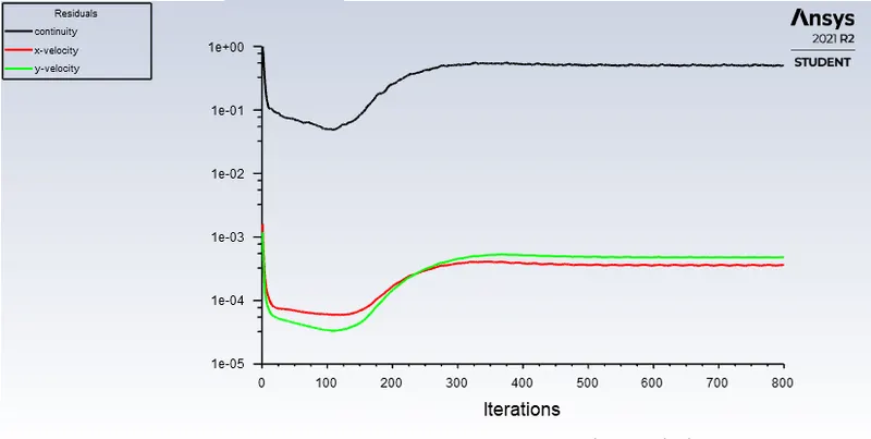
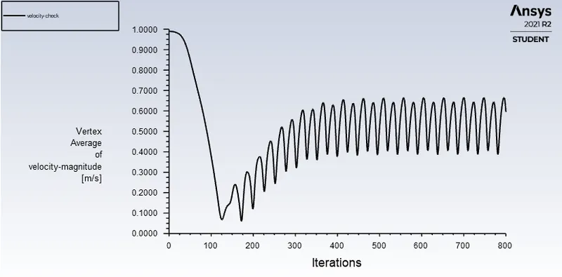
Steady

Residual plot

Velocity plot

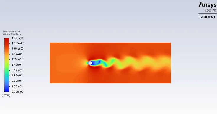
Velocity Contour

Transient

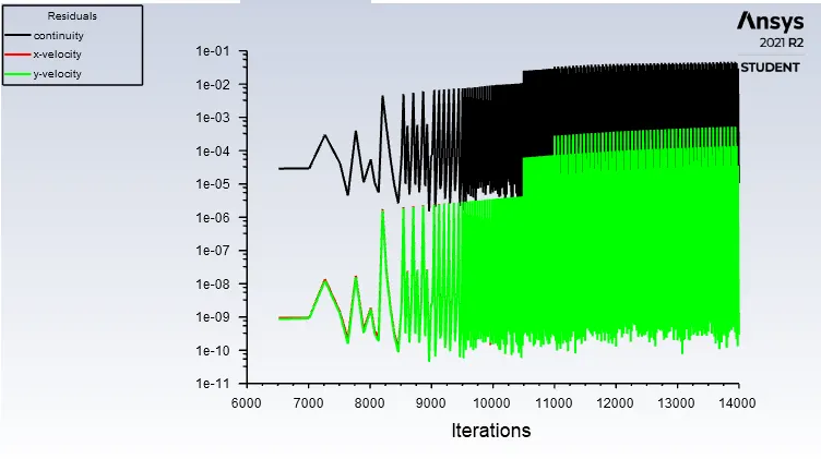
Residual plot

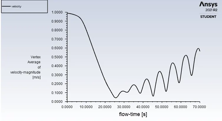
Velocity plot

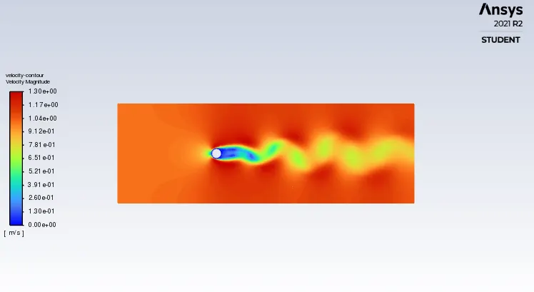
Velocity contour

Strouhal number:

Results>Plot>FFT> X- St number, Y-magnitude> plot FFT

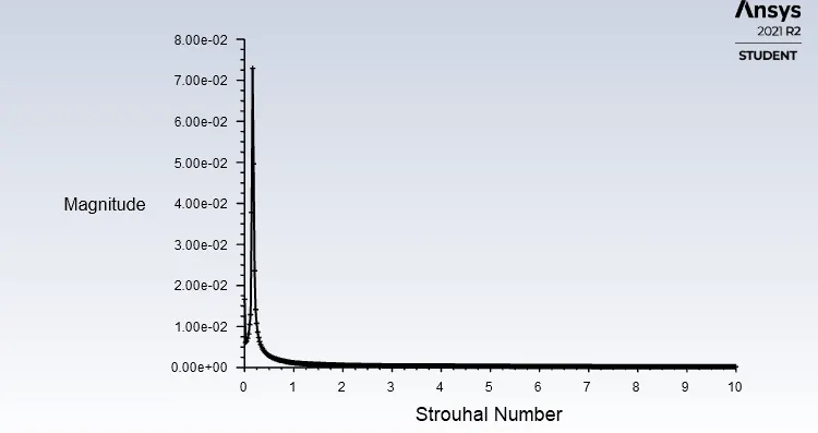
Write FFT> Save the file to a location you want> open in notepad

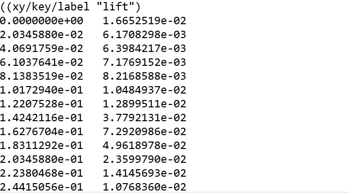
Here, you can see the magnitude is 0.0729 (Y-axis), and the corresponding Strouhal number (X-axis) is 0.1627.

St= 0.1627

Part-2

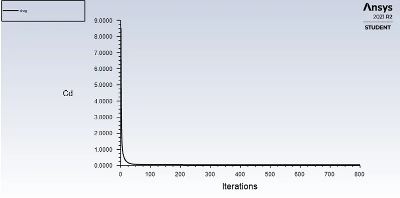
Steady Solver,

Case 1

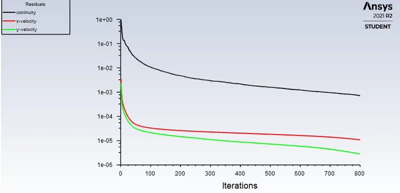
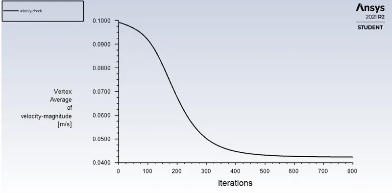
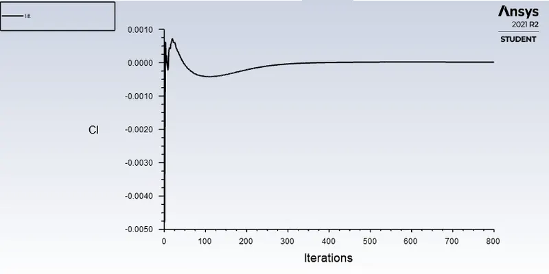
Re= 10

Velocity = 0.1 m/s

Residual plot

Velocity plot

Lift plot

Drag plot

Velocity contour

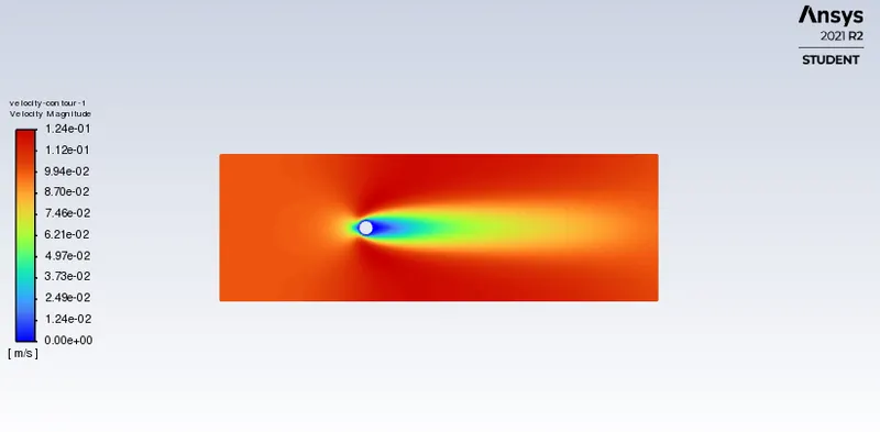
Case 2

Re = 100

Velocity= 1 m/s

Residual Plot

Velocity plot

Lift plot

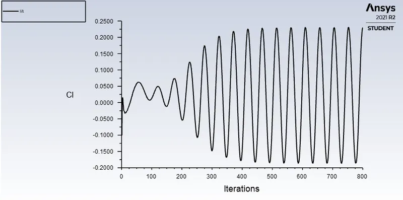
Drag plot

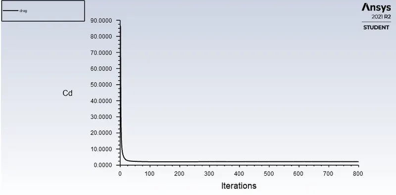
Velocity contour

Case 3

Re = 1000

Velocity = 10 m/s

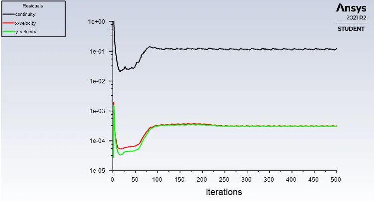
Residual Plot

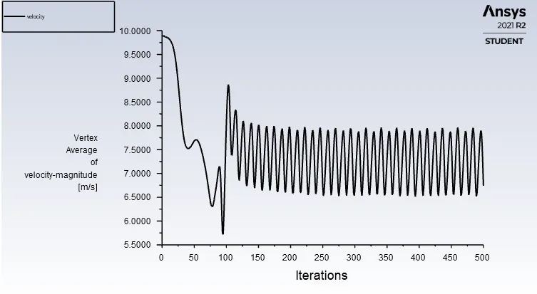
Velocity plot

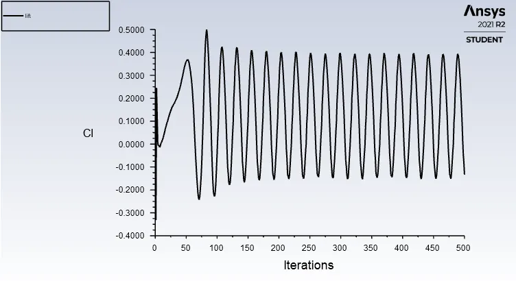
Lift plot

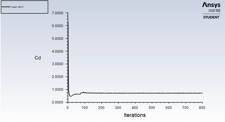
Drag plot

Velocity contour

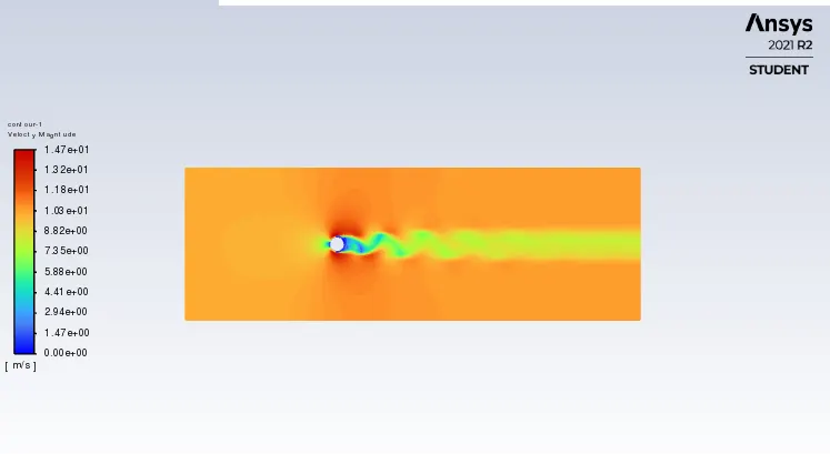
Case 4

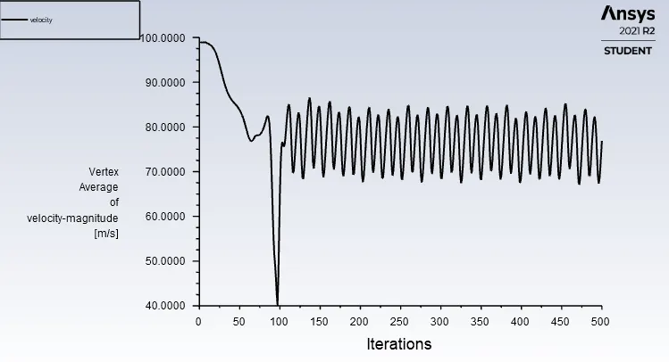
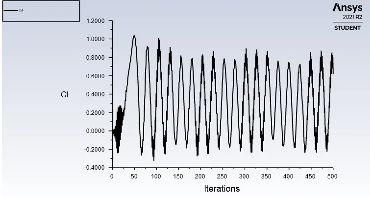
Re= 10000

Velocity = 100 m/s

Residual Plot

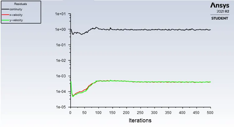
Velocity plot

Lift plot

Drag plot

Velocity contour

Case 5

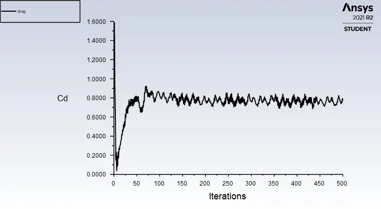
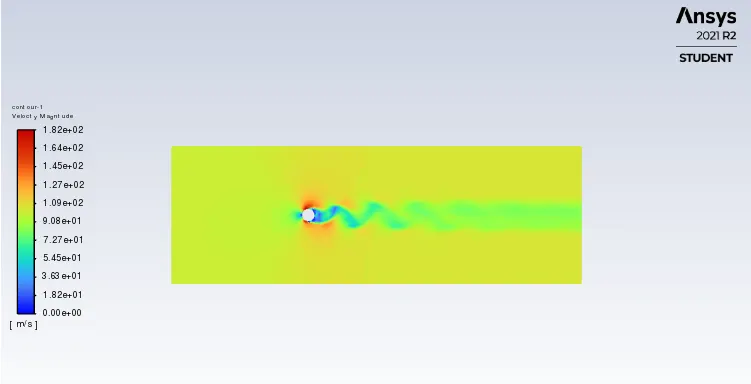
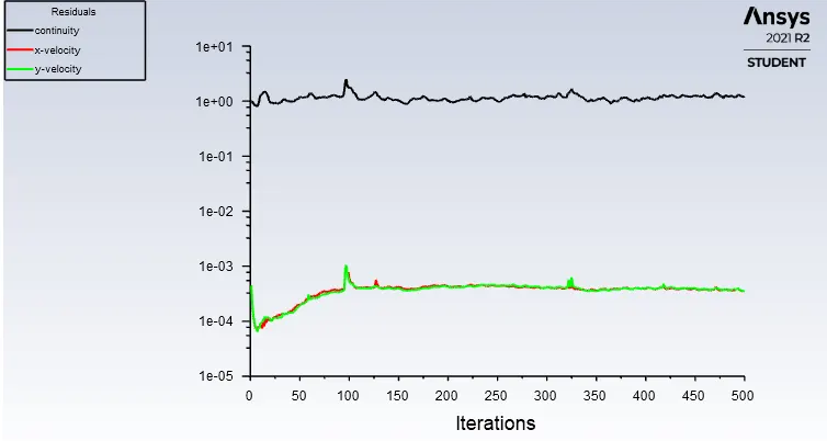
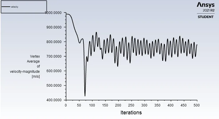
Re = 100000

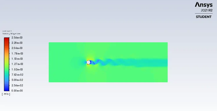
Velocity = 1000 m/s

Residual Plot

Velocity plot

Lift plot

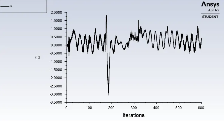
Drag plot

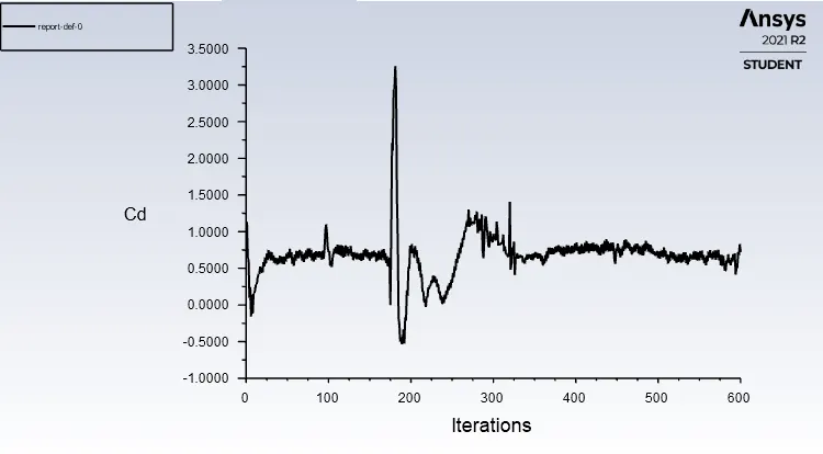
Velocity contour

Effect of Reynolds number on drag coefficient

Reynolds no	Cd
10	3.3
100	1.339
1000	0.733
10000	0.726
100000	0.580

Conclusion

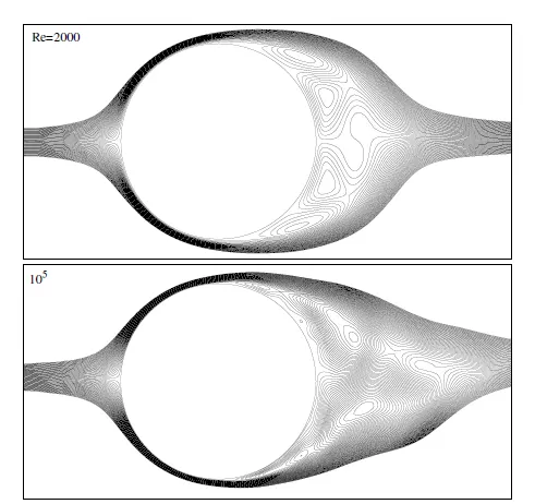
• It was observed that the coefficient of drag decrease with an increase in Reynolds number as the inertial force overcomes viscous force.
• For low Reynolds number, the viscous force is dominating one and there is the formation of laminar boundary layer and the flow separation starts at an angle less than 90 degrees hence the cd value is more.
• for higher Reynolds number, there is the formation of turbulent boundary layer and as the incoming air kinetic energy is more, therefore the inertial forces delay the flow separation and hence cd decreases with increase in Reynolds number (below figure). [4]

References:

[1] https://en.wikipedia.org/wiki/K%C3%A1rm%C3%A1n_vortex_street

[2] https://en.wikipedia.org/wiki/Strouhal_number

[3] B.N Rajani, S. Majumdar, A. kandasamy, Numerical simulation of flow over the cylinder, Applied Mathematical modeling 33, 2009.

[4] S.P Singh, S Mittal, "flow past a cylinder: Shear layer instability and drag crisis", IIT Kanpur, UP 208 016.