Week 5 - Rayleigh Taylor Instability

Rayleigh Taylor Instability

Aim:

To perform Rayleigh Taylor instability simulation for two fluids (i.e. Air and water) with different density, using volume of fraction method.

1. Compare the animation for different mesh size.
2. Run one more simulation with water and user-defined material(density = 400 kg/m3, viscosity = 0.001 kg/m-s) for refined mesh.

Introduction:

Rayleigh Taylor instability

The Rayleigh–Taylor instability is an instability of an interface between two fluids of different densities which occurs when the lighter fluid is pushing the heavier fluid. Examples include the behavior of water suspended above oil in the gravity of Earth.

Water suspended atop oil is an everyday example of Rayleigh–Taylor instability, and it may be modeled by two completely plane-parallel layers of immiscible fluid, the denser fluid on top of the less dense one and both subject to the Earth's gravity. The equilibrium here is unstable to any perturbations or disturbances of the interface: if a parcel of heavier fluid is displaced downward with an equal volume of lighter fluid displaced upwards, the potential energy of the configuration is lower than the initial state. Thus the disturbance will grow and lead to a further release of potential energy, as the denser material moves down under the (effective) gravitational field, and the less dense material is further displaced upwards. This was the set-up as studied by Lord Rayleigh. [1]

Atwood number

The Atwood number (A) is a dimensionless number in fluid dynamics used in the study of hydrodynamic instabilities in density stratified flows. It is a dimensionless density ratio defined as,

`A=(ρ_1-ρ_2)/(ρ_1+ρ_2 )`

where,

`ρ_1=`density of heavier fluid

`ρ_2=`density of lighter fluid

Some practical CFD models based on the mathematical analysis of Rayleigh Taylor waves:

Richtmyer–Meshkov instability

The Richtmyer–Meshkov instability (RMI) occurs when two fluids of different density are impulsively accelerated. Normally this is by the passage of a shock wave. The development of the instability begins with small amplitude perturbations which initially grow linearly with time. This is followed by a nonlinear regime with bubbles appearing in the case of a light fluid penetrating a heavy fluid, and with spikes appearing in the case of a heavy fluid penetrating a light fluid.

Kelvin-Helmholtz instability:

The Kelvin–Helmholtz instability occurs when there is velocity shear in a single continuous fluid or a velocity difference across the interface between two fluids. Kelvin-Helmholtz instabilities are visible in the atmospheres of planets and moons, such as in cloud formations on Earth or the Red Spot on Jupiter, and the atmospheres (coronas) of the Sun and other stars.

PROCEDURE:

Pre-Processing:

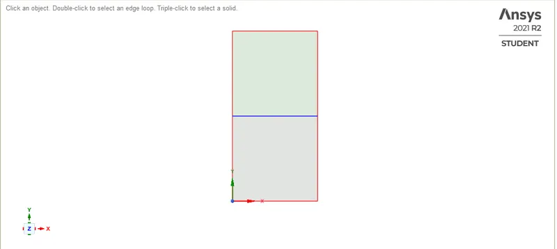
Geometry

Mesh

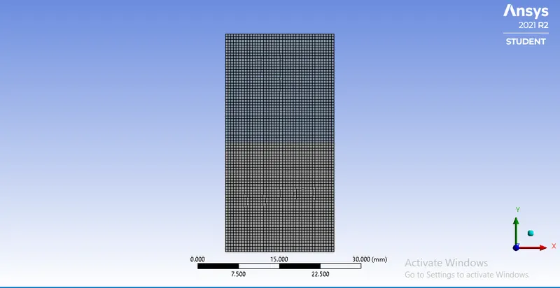
Elements size: 0.5mm

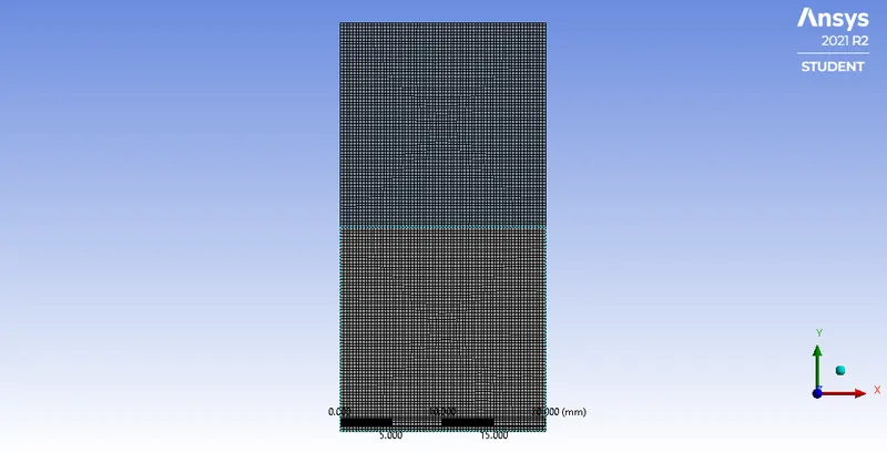
Element size: 0.3mm

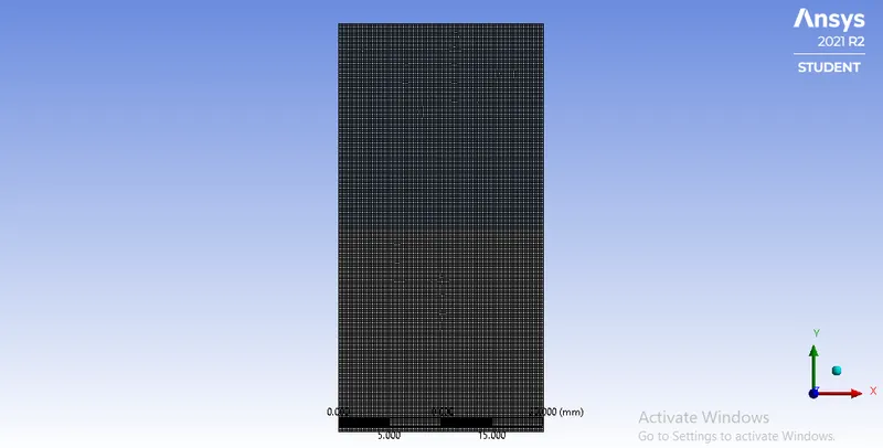
Element size: 0.2mm

Setup

Transient:

General: Pressure based, absolute, Transient state

Gravity: x=0, y—9.81, z=0.

Model: Laminar

Multiphase: volume of fluid

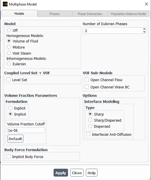
Material: fluid, (air)

Density = 1.225 kg/

Viscosity = 0.00001987 kg/ms

Fluid, (water)

Density = 998 kg/

Viscosity = 0.001003 kg/ms

Fluid, (User-defined)

Density = 400 kg/

Viscosity = 0.001 kg/ms

Phases:

Cell zone: fff_air_surfaces

Fff_water_surfaces

Method: Simple

Initialization: Hybrid initialization

Patch:

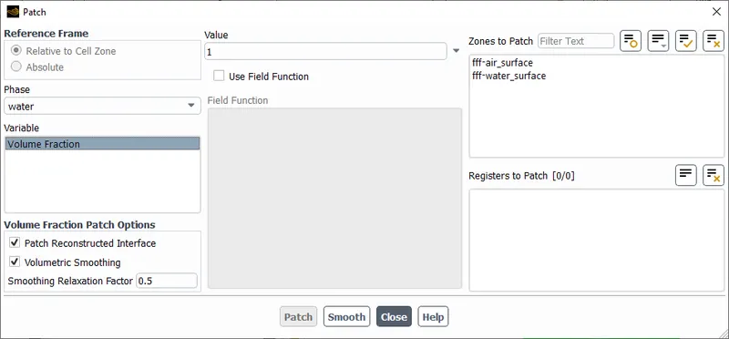
Run-calculation: 400-iterations

Results

Post-Processing

Case1

Mesh size= 0.5mm

Primary fluid= air

Secondary fluid= water

Time step=0.005

Link: https://drive.google.com/drive/folders/1ynbU5n71yF6H-7iAGb1odeK3qh58fndm?usp=sharing

Case2

Mesh size= 0.3mm

Primary fluid= air

Secondary fluid= water

Time step=0.005

Link: https://drive.google.com/drive/folders/1l-EPgGM-NZrynioVYkkMcyz5-_N_6gfr?usp=sharing

Case3

Mesh size= 0.2mm

Primary fluid= air

Secondary fluid= water

Time step=0.005

Link: https://drive.google.com/drive/folders/1Z_vok9BHyDawGK2POB7zLaMYq9wqZdvQ?usp=sharing

Case4

Mesh size= 0.2mm

Primary fluid= air

Secondary fluid= User-defined

Time step=0.005

Link: https://drive.google.com/drive/folders/1RGjPdyZNpgmExaYQExnR1V4b_4sX2Xnu?usp=sharing

Atwood number:

Case 1, 2 and 3

`ρ_1= 998 kg/m^3 , ρ_2= 1.225 kg/m^3`

`A=(ρ_1-ρ_2)/(ρ_1+ρ_2 )=(998-1.225)/(998+1.225)=0.9975`

Case 4

`ρ_1= 998 kg/m^3, ρ_2= 400 kg/m^3`

`A=(ρ_1-ρ_2)/(ρ_1+ρ_2 )=(998-400)/(998+400)=0.4278`

Conclusion

• In mesh independence study, it was observed that with 0.2mm element size we got much accurate and refined result as compared to 0.5mm. The patterns were clearly visible in 0.2mm (animation file), whereas the patterns were blurring in 0.5mm mesh (animation file).
• Steady state approach is not valid because, instability problems are generally simulated using transient state inorder to observe the mixing layer patterns.
• Higher Atwood number represent that there is higher density difference which results in higher rate of mixing of two fluids, and lower Atwood number represent that there is lower density difference and hence lower rate of mixing of two fluids (which can be properly observed in videos).

References:

[1] https://en.wikipedia.org/wiki/Rayleigh%E2%80%93Taylor_instability