Week 1- Mixing Tee
Mixing Tee Simulation
Aim:
- To carry out steady-state simulations to compare the mixing effectiveness when hot and cold inlet temperatures are 36℃ and 19℃ respectively.
- Case1
- Short mixing tee with a hot inlet velocity of 3m/s
- Momentum ratio of 2,4
- Case 2
- Long mixing tee with a hot inlet velocity of 3m/s
- Momentum ratio of 2,4
- To perform k-epsilon and k-omega SST model for one of the above cases and accordingly choose the suitable model for remaining cases.
- To perform mesh independent study for any of the above cases.
Introduction:
A mixing tee is a device used to mix two fluids at two different temperatures in order to get the desired temperature at the output. It has two inlets one cold along Y-axis and a hot inlet along X-axis, and the corresponding outlet is along X-axis.
Applications, where pipeline mixing with tees are used, include low viscosity mixing such as wastewater treatment and blending of some oils (injection of additives) and petrochemical products. Other applications include the blending of fuel gas and the mixing of feed streams for catalytic reactors. [1]
Formulations:
Momentum ratio:`V_(c_i )/V_(h_i )`
`T_mixture=(m_h*T_(h_i )+m_c*T_(c_i ))/(m_h+m_c )`
Where,
`V_(c_i )` = cold inlet velocity
`V_(h_i )` = hot inlet velocity
`m_h`= mass flow rate of hot inlet
`m_c`= mass flow rate of cold inlet
`T_(h_i )`= temperature of hot inlet
`T_(c_i )` = temperature of cold inlet
Approach and solving:
The experiment was performed in 8 simulations,
- 2 simulations for mesh independent study in order to choose a suitable element size for simulation.
- 2 simulations for k-epsilon and k-omega for each case in order to choose the suitable model for simulation.
- 4 simulations for Case 1 and Case 2 for different momentum ratios.
First I performed a mesh independent study for element sizes 5mm and 3mm, followed by selecting the suitable model for simulation, and then after having the suitable element size and model I performed simulation for both Case 1 and Case 2.
Mesh Independent Study:
- Case 1, momentum ratio 2:
|
Element size |
5mm |
3mm |
|
No of elements |
14166 |
39375 |
- Mesh: In layman's terms, meshing is nothing but dividing the complete body into small parts and on which our analysis takes place. There are different types of mesh depending upon shapes and size.
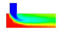
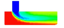
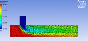
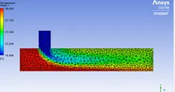
(a) 5mm (b)3mm
- From mesh independent study it was found that as the element size decreases from 5mm to 3mm the number of elements on the object increases and hence we get a more refined output as we can see in the above figure.
- Hence, I have selected a 3mm mesh for my simulation part. (As less than 3mm was not compatible with the student version of ANSYS).
K-epsilon and K-omega model
In order to solve the governing equations of mass, continuity, energy, and viscous equation, there are different models for how the turbulence is being captured. K-epsilon and k-omega are RANS-based turbulence models (Reynolds Average Navier-stokes).
K-epsilon:
- Case 1 momentum ratio 2
- K-epsilon > Relizable > standard wall function,
Output temperature graph
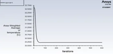
Fig (5)
The standard deviation of output temperature
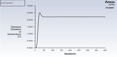
Fig (6)
K-omega:
- Case 1 momentum ratio 2
- K-epsilon > SST >production limiter,
Output temperature graph
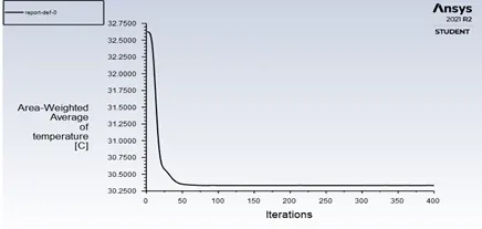
Fig (7)
The standard deviation of output temperature
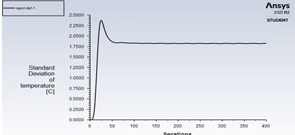
Fig (8)
From the above observations, (Fig 5 to Fig 8)
|
K-epsilon |
K-omega |
|
|
Output temp (℃) |
30.25 |
30.325 |
|
Deviation of output temperature (℃) |
2.25 |
1.75 |
`T_mixture=(m_h*T_(h_i )+m_c*T_(c_i ))/(m_h+m_c ) = ((0.0009*3)*36 +(0.0002*6)*19)/((0.0009*3)+(0.0002*6)) = 30.76℃` ……(theoretical calculation)
Where `m=ρ*A*V`
- %error of output temperature,
- K-epsilon-65%
- K-omega – 1.414%
[Note: we know that less the standard deviation good mixing and more the standard deviation bad mixing.]
Hence we can say K-omega gives the more precise and desired output as the standard deviation of output temperature of K-omega is less than K-epsilon, and also the percentage error of output temperature is less for K-omega as compared to K-epsilon.
PROCEDURE:
- Geometry
- Mesh
- Setup
- Solution
- Results
Pre-Processing:
Case 1: Short Mixing Tee
Geometry
- Raw model:
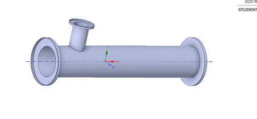
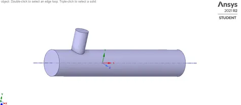
- Fluid volume extraction > Suppress for physics
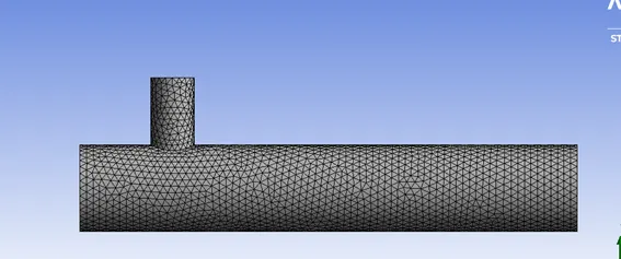
Meshing:
- Element size = 3mm
- No of nodes = 8289
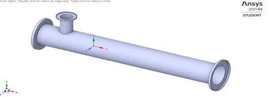
Case 2: Long Mixing Tee
Geometry
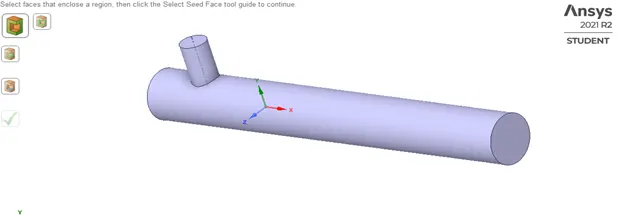
- Raw model:
- Fluid volume extract > Suppress for physics
Meshing
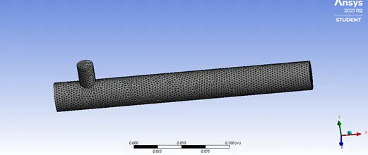
- Element size = 3mm
- No of nodes = 11639
- The Solid works file of the model was imported to Spaceclaim.
- As our fluid will flow through the volume of pipe the volume extraction was done from the prepare menu by selecting the edges and was suppressed for physics.
- We then named the hot inlet, cold inlet, outlet, and walls of the pipe, and then we performed the tetrahedral meshing by keeping the element size to 3mm.
Setup: this is the main step in analysis because according to our input conditions the simulation will run.
- The simulation was run in steady-state
- Model selected was k-omega > SST > production limiter
- Working fluid was selected as an air
- Inlet velocity and temperatures were given,
Case 1:
- Velocity at hot inlet = 3m/s
- The temperature at hot inlet = 36 ℃
- Temperature at cold inlet = 19 ℃
- Momentum ratio = 2,4
Case 2:
- Velocity at hot inlet = 3m/s
- Temperature at hot inlet = 36 ℃
- Temperature at cold inlet = 19 ℃
- Momentum ratio = 2,4
- Now under the results, we define the reports for standards deviation of output temperature and weighted average temperature under surfaces.
- We then initialized by using hybrid initialization.
- And run the calculation for 400 iterations and the results were calculated.
Results
Post-Processing
Case 1
Momentum ratio: 2
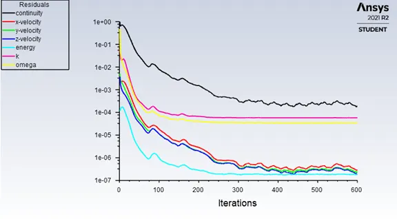
Residual graph: Converge at 125 iteration
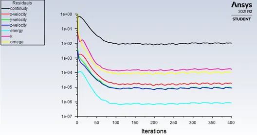
Velocity of hot inlet= 3m/s
Velocity of cold inlet= 6m/s
Contour plots:
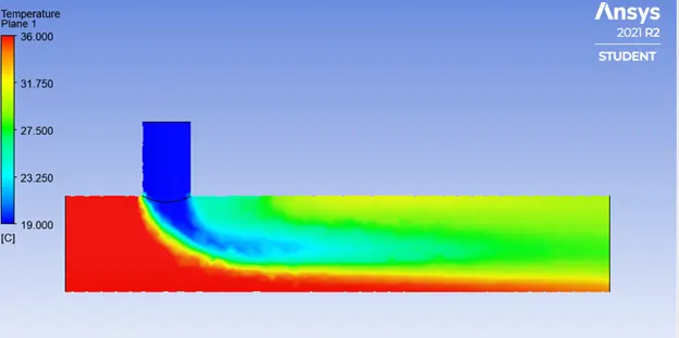
- The temperature along the length of the pipe
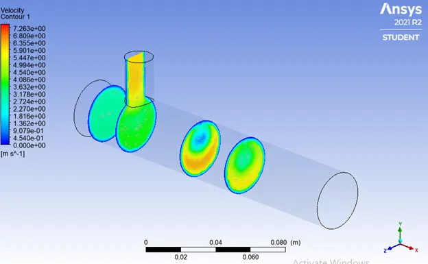
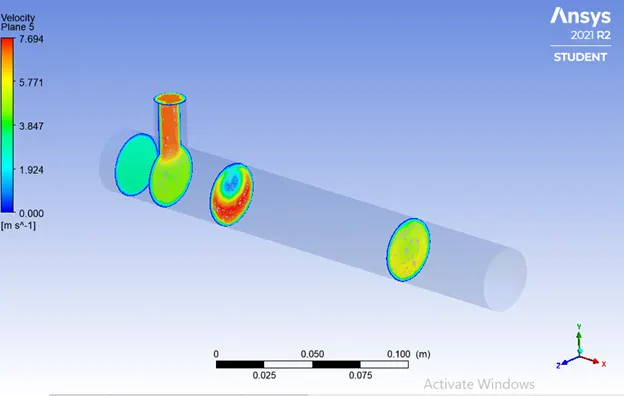
- Velocity along the length of pipe
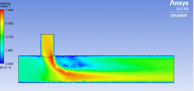
- Temperature across the length of pipe
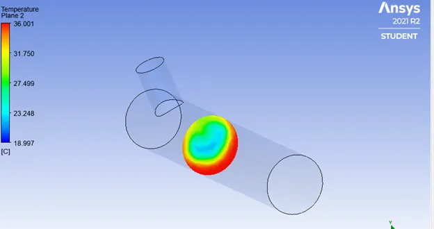
- Velocity across the length of pipe
Line plots:
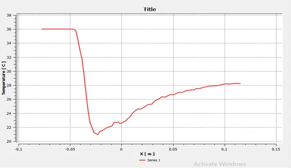
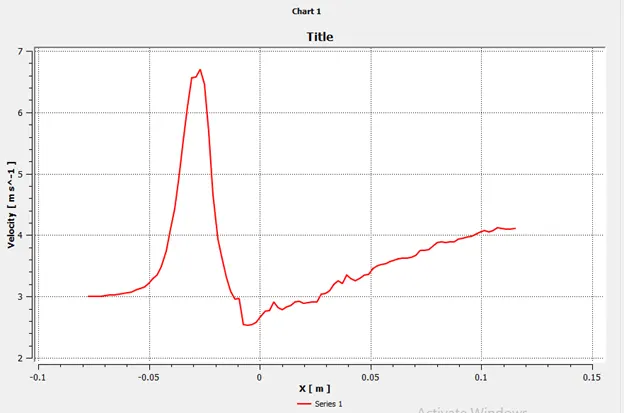
- The temperature along the length of pipe
- Velocity along the length of pipe
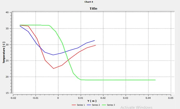
- Temperature across the length of pipe
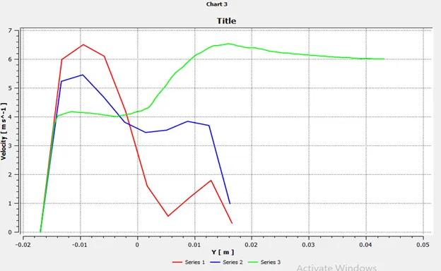
- Velocity across the length of pipe
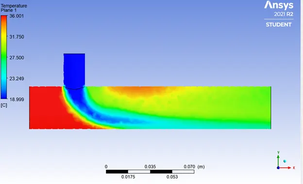
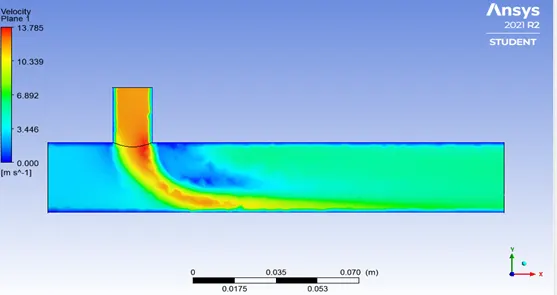
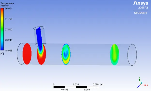
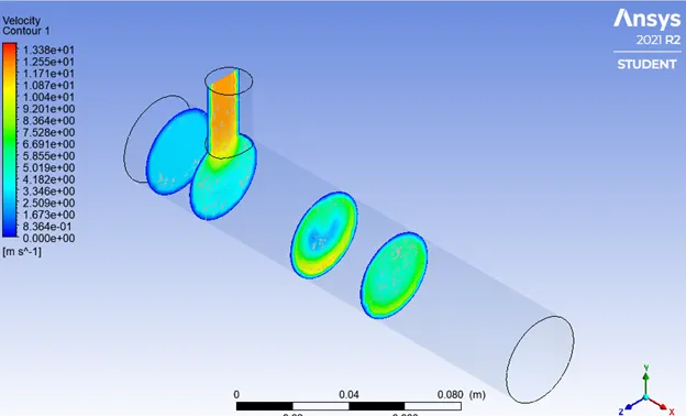
Momentum ratio: 4
Residual graph: Converge at 400 iteration
Velocity of hot inlet= 3m/s
Velocity of cold inlet= 12m/s
Contour plots:
- The temperature along the length of the pipe
- Velocity along the length of pipe
- Temperature across the length of pipe
- Velocity across the length of pipe
Line plots:
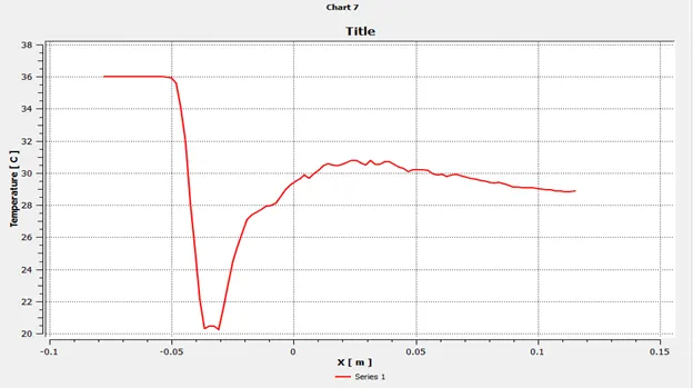
- The temperature along the length of the pipe
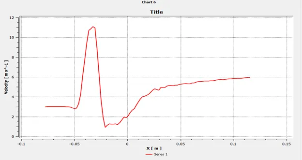
- Velocity along the length of pipe
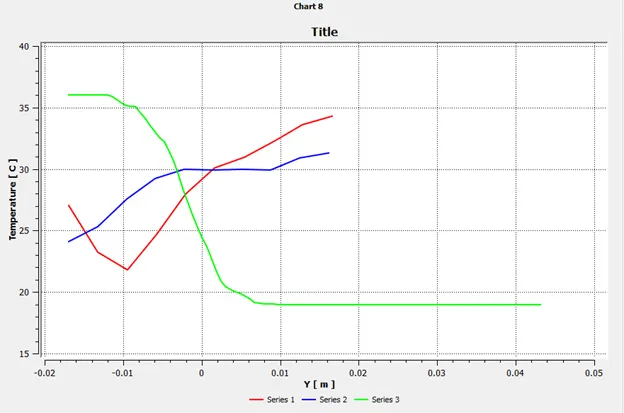
- Temperature across the length of pipe
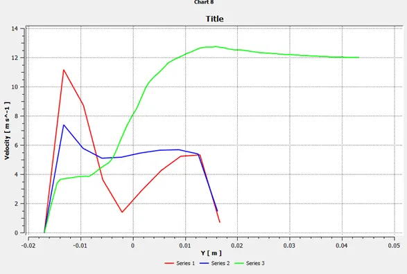
- Velocity across the length of pipe
Case 2
Momentum ratio: 2
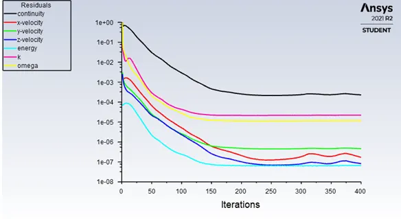
Residual graph: Converge at 200 iteration
Velocity of hot inlet= 3m/s
Velocity of cold inlet= 6m/s
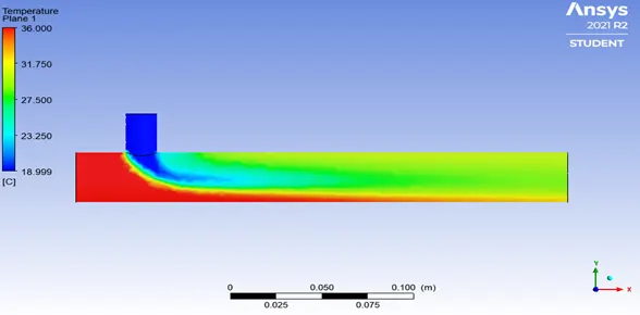
Contour plots:
- The temperature along the length of the pipe
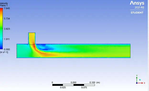
- Velocity along the length of pipe
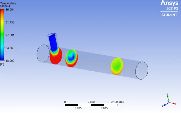
- Temperature across the length of pipe
- Velocity across the length of pipe
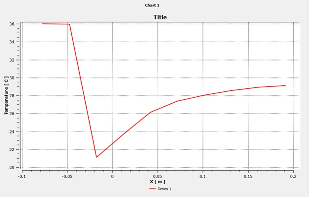
Line plots:
- The temperature along the length of the pipe
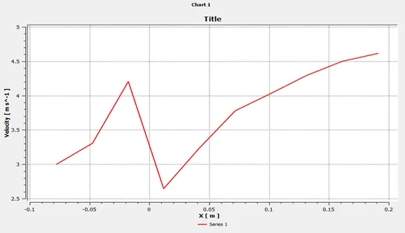
- Velocity along the length of pipe
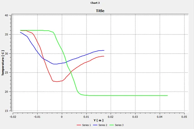
- Temperature across the length of pipe
- Velocity across the length of pipe
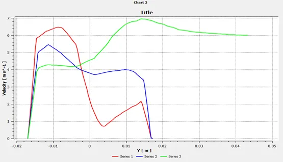
Momentum ratio: 4
Residual graph: Converge at 300 iteration
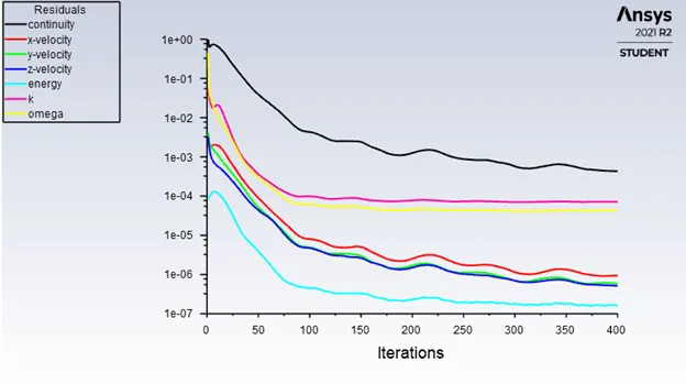
Velocity of hot inlet= 3m/s
Velocity of cold inlet= 12m/s
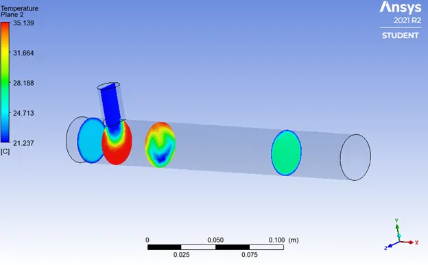
Contour plots:
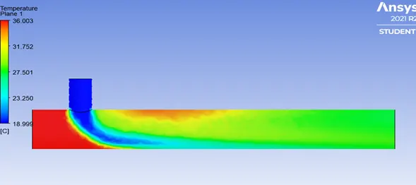
- The temperature along the length of the pipe
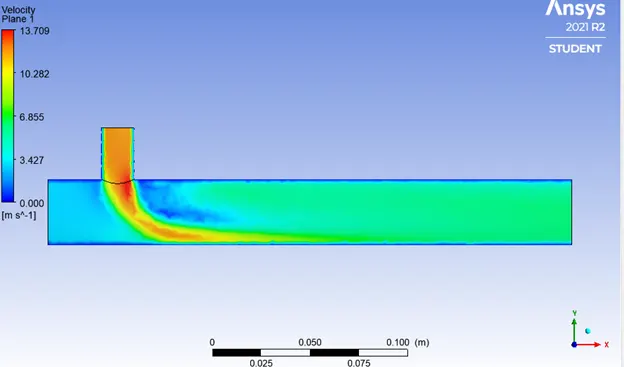
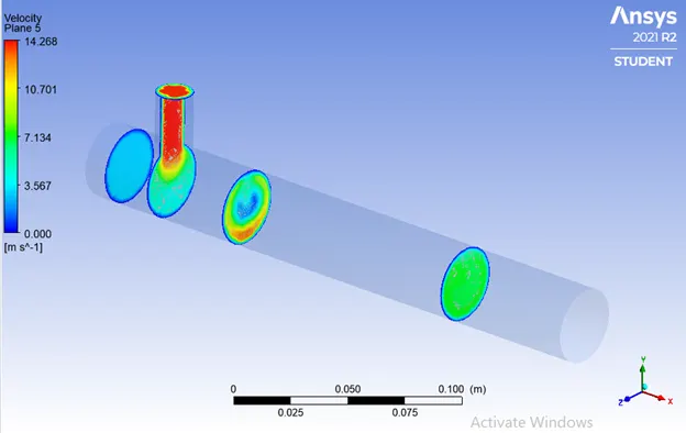
- Velocity along the length of pipe
- Temperature across the length of pipe
- Velocity across the length of pipe
Line plots:
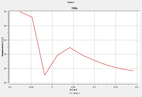
- The temperature along the length of the pipe
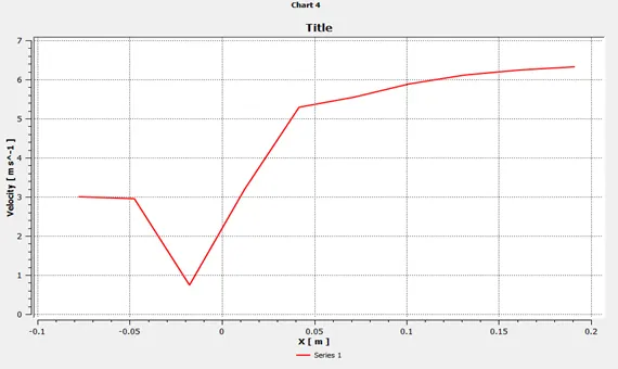
- Velocity along the length of pipe
- Temperature across the length of pipe
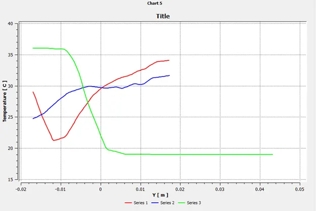
- Velocity across the length of pipe
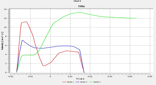
Conclusion:
From the above results, we can conclude that,
- In the fluid flow along the length of the pipe, the temperature at the mixing region drops to the near low value of the cold inlet temperature and due to mixing, we get the average temperature at the output.
- In the fluid flow along the length of the pipe, we can observe that the velocity of the cold inlet decreases at the mixing region and then starts to average as it reaches the outlet.
- Since the wall is in the no-slip condition the velocity is zero at the walls and the velocity increases as we move towards the center of the pipe.
- As the mass flow rate and temperature of the hot inlet are more as compared to the cold inlet the average temperature at the outlet is more towards the hot region.
Table of comparison for cell count, outlet temperature, No of iterations for convergence:
|
|
Case 1 |
Case 2 |
||
|
6m/s |
12m/s |
6m/s |
12m/s |
|
|
Cell count |
39375 |
39375 |
56003 |
56003 |
|
Avg outlet temperature |
30.325 |
27.625 |
30.325 |
27.625 |
|
No of iterations for convergence |
125 |
400 |
200 |
300 |
- It is observed that the outlet temperature is independent of the length for both the cases
- And as the momentum ratio increases the temperature at the output was found to decrease about 3℃ for both the case.
References: