Week 8 - Simulating Cyclone separator with Discrete Phase Modelling
Aim: To perform analysis on cyclone separator and calculate the separation efficiency and pressure drop.
Objective:
- To perform analysis on a given cyclone separator by varying the velocity from 1 m/s to 5 m/s with particle size 5 micrometer and calculate separation efficiency and pressure drop.
- To perform analysis on a given cyclone separator by varying the particle size from 1 to 5 micrometer with a velocity of 3 m/s and calculate separation efficiency and pressure drop.
Introduction
What is cyclone separator ??
Cyclone separators are basically centrifugal separators.
There is tangential inlet and axial discharge.
classified as two types
1)Cyclone Separator: Used to separate liquids and solids from the gas stream.
2)Hydrocyclones: Used to separate liquids or separate one liquid from other.
Principle:
Inertial forces are generated by the velocity of the incoming fast-moving stream of the feed the rotational action of the inlet stream crates a centrifugal force and descends in a helical path on the inside of the cylindrical portion more dense particles are thrown out of the mainstream and collected from the bottom, smaller particles may be carried away by fast-moving fluid or air from the outlet upward in the column.
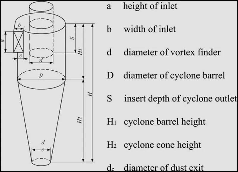
Fig: Cyclone Separator
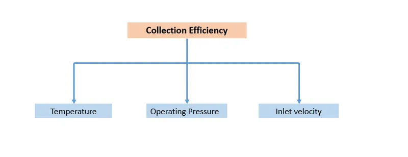
Collection efficiency depends on temperature, operating pressure, and inlet velocity.
Separation Efficiency=1 - Collection efficiency
There are various empirical models for calculating the collection efficiency of Cyclone Separator.
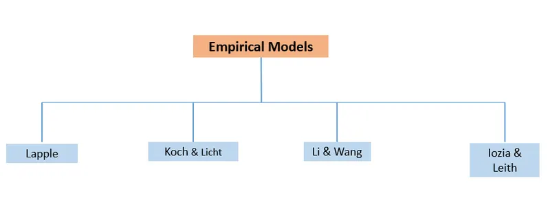
Lapple Model:
Lapple Model was developed by Force balance without considering the Flow Resistance. The assumption of this model is that particles entering in the separator are evenly distributed at the inlet.The particle that travel inlet- half width to the wall is collected with 50% efficiency.The empirical relationship developed by Lapple to calculate 50% cut diameter is
`d_{pc}=[(9*mu*b)/(2*pi*N_{e}*v_{i}(rho_{p}-rho_{g}))]^(1/2)`
where `N_{e}="number of revolutions"`
`N_{e}=(1/a)[H1+(H-H_{1})/(2)]`
Efficiency of collection
`eta_{i}=1/(1+(d_{pc}+d_{"pi"})^2)`
Iozia and leith:
The model assumes that particle carried by the vortex endures influences of two forces 1)centrifugal force,Z 2)flow resistance,F. The collection efficiency is given by
`eta_{i}=1/(1+(d_{pc}+d_{"pi"})^beta)`
where
`beta=0.62-0.87*ln(d_{pc}/100)+5.21*ln((a*b)/D^2)+1.05*[ln((a*b)/D^2)]^2`
`d_{pc}=50% "cut size given by barth"`
Li & Wang Method
The Lin and Wang method includes particle bounce or reentrainment and turbulent diffusionat the cyclone wall.A two dimensional analytical expression of distribution in the cyclone is obtained.
Assumptions:
1)The radial particle velocity and radial concentration are not constant for uncollected particles within the cyclone.
2)Boundary condition for turbulence diffusion coefficient and particle bounce reentrainment are `c=c_{0} "at " theta=0`
`eta_{i}=1-exp(-lamda*theta_{1})`
where
`theta_{1}=2*pi*((S+L)/a)`
Koch and litch model:
This theory recognises the inherent turbulent nature of the cyclone and the distribution of gas resident time in cyclone,koch and litch described the particle motion in the entry and collection regions with following assumptions
1)Tangential velocity of the particle is equal to tangential velocity of gas flow,so there is no slip in the gas and particle in tangential direction
2)The tangential velocity is related to radius of the cyclone `u*R^n="constant"`
Cut-Off size
Cyclones have been characterised by the cut-off size which is defined as particle size for which the cyclone collection efficiency is 50%.
Setting up The geometry in SpaceClaim
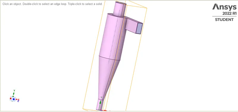
The fluid volume is extracted from the model by edge selection.
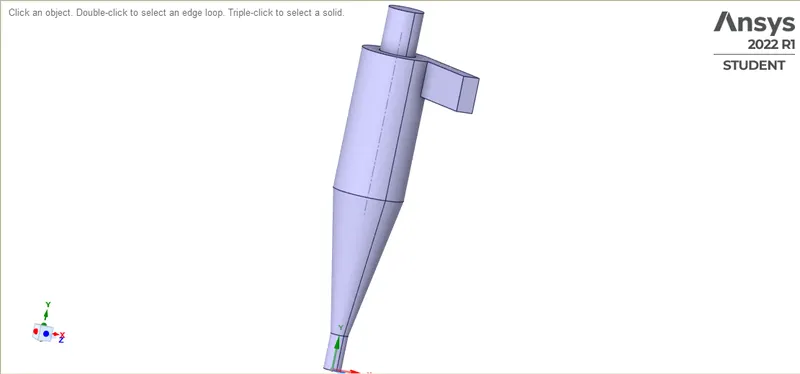
Dimesions of the spaceclaim geometry
`a=100 mm,b=50mm,d=104mm,D=200mm,S=125mm,H_{1}=400mm ,d_{c}=50mm , H_{2}=406.9705 mm`
Meshing
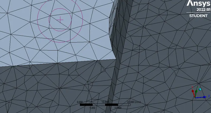
Mesh
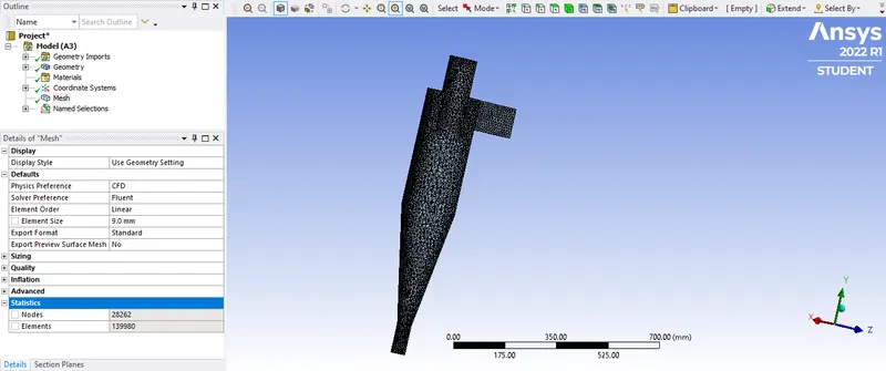
Cutshell Mesh
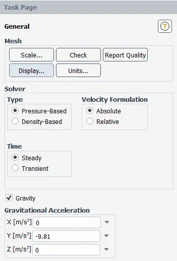
SOLVER SETUP
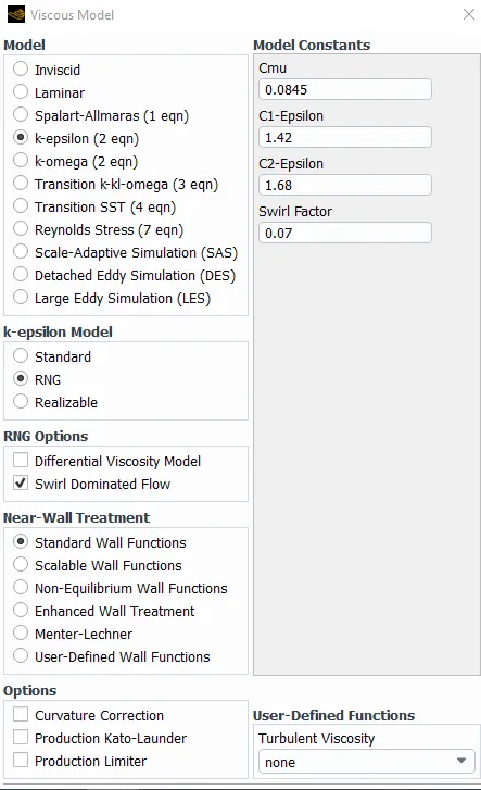
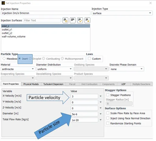
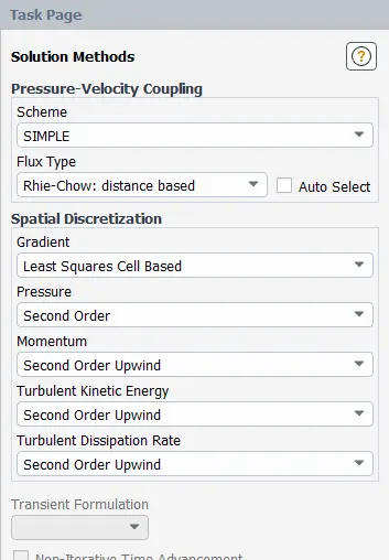
Boundary conditions :
Inlet: Reflect
Wall: Reflect
outlet top: Escape
Outlet Bottom: Trap
SIMULATION RESULTS
particle velocity =1m/s
particle size= 5 micrometer



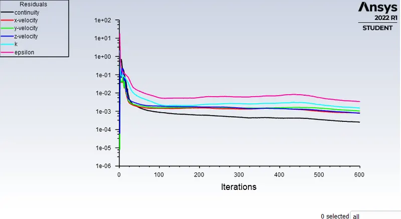
Scaled Residuals
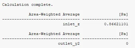
Area_Weighted Pressure at inlet
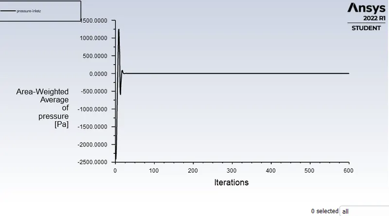
From the plots of residuals and area weighted average pressure we can conclude that solution is converged for 600 iterations.
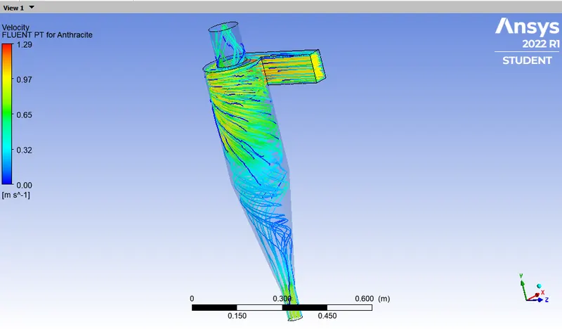
Velocity Contour
Pressure Contour
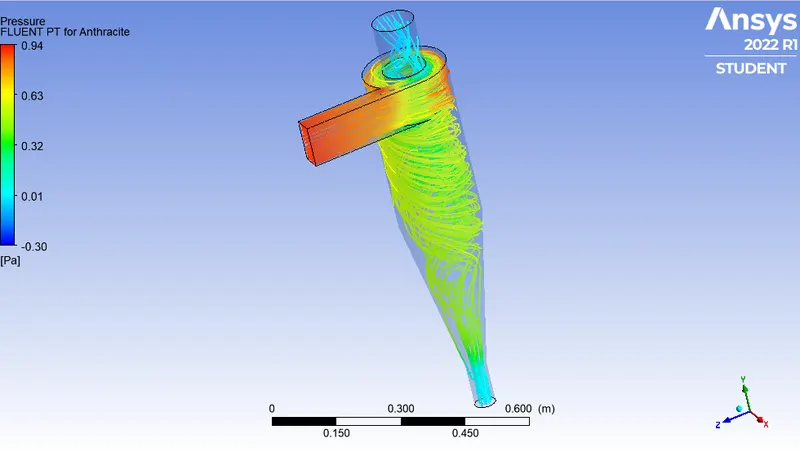
Particle Tracking animation link
Comparision from the simulation
| Particle Size | Particle Velocity | Particle Tracked | Particles Escaped | Particles Trapped | Incomplete | Seperation efficiency | Inlet pressure | Outlet Pressure | Pressure Drop |
| 5 micron | 1 m/s | 142 | 25 | 28 | 89 | 52.83018868 | 0.8662 | 0 | 0.8662 |
| 2m/s | 142 | 38 | 30 | 74 | 44.11764706 | 3.572 | 0 | 3.572 | |
| 3m/s | 142 | 46 | 32 | 64 | 41.02564103 | 8.13175 | 0 | 8.13175 | |
| 4m/s | 142 | 49 | 41 | 52 | 45.55555556 | 14.5531 | 0 | 14.5531 | |
| 5m/s | 142 | 43 | 55 | 44 | 56.12244898 | 23.1453 | 0 | 23.1453 | |
| 1 micron | 3 m/s | 142 | 55 | 65 | 22 | 54.16666667 | 23.21 | 0 | 23.21 |
| 2 micron | 142 | 54 | 70 | 18 | 56.4516129 | 23.21 | 0 | 23.21 | |
| 3 micron | 142 | 52 | 68 | 22 | 56.66666667 | 23.21 | 0 | 23.21 | |
| 4 micron | 142 | 51 | 66 | 25 | 56.41025641 | 23.21 | 0 | 23.21 | |
| 5 micron | 142 | 44 | 65 | 33 | 59.63302752 | 23.21 | 0 | 23.21 |
CONCLUSION
1)The separation efficiency is increasing with the particle size for constant velocity.
2)for the particle velocity from 1 to 3 m/s separation efficiency decreases than for 3 to 5 m/s separation efficiency increases.
3)pressure drop increases for increasing the particle velocity.
4)for constant velocity pressure drop is constant for all the cases.