Week 3 - Solving second order ODEs

%solving the second order differential equation
%the system is the damped pendulum
clear all
close all
clc

%geometric properties of pendulum
      b=0.05;%damping factor
      g=9.81;%gravitational acceleration
      l=1; %length of pendulum
      m=1; %mass of the pendulum
   
      
      
      %initial condition 
    theta_0=[0;3];   %column matrix the first value is displacement and second value is velocity
    t_span=linspace(0,20,300);  %time span for the integration is 0 to 20 seconds
   
    
    %calling the ode function 
    
    [t,results]=ode45(@(t,theta) pendulumodefun(t,theta,b,g,m,l),t_span,theta_0);
    dtheta1_dt=results(:,1); %assingning the variable to the angular displacement vector 
    dtheta2_dt=results(:,2); %assingning the variable to the angular velocity vector 
    subplot(2,1,1); %dividing the figure 1 into 2 raws and ploting displacement and velocity
    plot(t,dtheta1_dt)
    xlabel('time')
    ylabel('angular displacement')
    subplot(2,1,2);
    plot(t,dtheta2_dt,'color','r')
    xlabel('time')
    ylabel('angular velocity')
     
    
    %for the animation of the pendulum
figure(2)
                 ct=1;
                 
                 for i=1:length(t_span)%introducing the for loop for takingt the time value and calculate the position of the pendulum for each time 
                   
                     
                     x0=0;                %fixed end of the pendulum
                     y0=0;                %fixed end of the pendulum
                     
                     
                     x1=l*sin(dtheta1_dt(i));         %x position of the pendulum for the time value 
                     y1=-l*cos(dtheta1_dt(i));         %y position of the pendulum for the time value
                     
                     
                     figure(2)
                     
                     plot([-0.3 0.3],[0 0],'linewidth',5);  %plotting the fixed end support 
                     hold on                                 %hold on for the each time step 
                     
                     plot([x0 x1],[y0 y1],'linewidth',3);     %plotting the  pendulum rope
                     plot(x1,y1,'marker','O','markersize',15,'markerfacecolor','b')    %plotting the bob 
                     hold off                                 %hold off the previous time step plot for the next time step
                     
                     axis([-2 2 -2 2])        %fixed axis so that the axis does not change with each time frame
                     grid on
                     pause(0.001) 
                     M(ct)=getframe(gcf);
                     ct=ct+1;
                 end
    
movie(M)
videofile=VideoWriter('pendulum_script.avi','uncompressed AVI');
open(videofile)
writeVideo(videofile,M)
close(videofile)

pendulumodefun to solve the second order differential equation

function [dtheta_dt]=pendulumodefun(t,theta,b,g,m,l)
theta1=theta(1);
theta2=theta(2);
dtheta1_dt=theta2;
dtheta2_dt=((-b/m)*theta2-(g/l)*sin(theta1));
[dtheta_dt]=[dtheta1_dt;dtheta2_dt];
end

Stepwise explanation of the code

1)first we clear all previous plots and variables by the command

2)geometrical properties of the pendulum is defined b,g ,l,m

3)initial angular displacement and angular velocity is defined as a column matrix

4)pendulum ode function is created in a separate Matlab program which will take inputs (time ,theta,b,g,l,m) and gives the output as [t, results]

Results is the matrix having the two columns the first column is the angular displacement and the second column is the angular velocity

5)plotting the graph for the angular displacement and angular velocity with the subplot of the two raws

6)the variable defined for step 1 and it will get increased every time the for loop is getting executed

7)for loop is introduced for taking the value of each time step and calculating the position of the pendulum at each time step

8)giving the second figure the name figure 2 to put it into the separate plot

9)making the video file and saving the file as avi format

ERRORS FACED DURING THE CODE

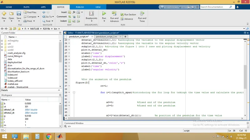
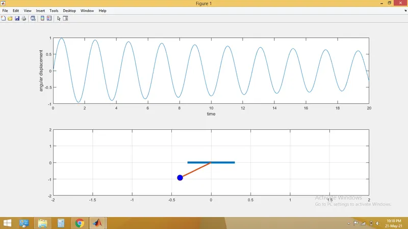
I have given the command of figure 2 before the for loop and it is disturbing my figure1 plot.

the animation video link of youtube

https://youtu.be/1JqdnXe2PiI