Week 4.1 - Genetic Algorithm

What is a genetic algorithm?

Basically, it is the technique to optimize the objective function by iteration. starts with the initial generation of candidate solutions and that are tested against the objective function.

The key idea is the “evolution is the optimization”

It uses the concept of evolutionary biology, the concept is the “the survival of the fittest”, Darwinian theory.

At each iteration, there is a progressive improvement of the objective.

Let’s say that we have the objective function Y as a function of x(1),x(2) so the genetic algorithm combines the values of x(1) and x(2) and finds the best solution.

GA search for the population of points not a single point.

GA uses the objective function information and not the second derivative or the first-order derivative

GA uses the stochastic transition rules not the deterministic rules, stochastic means probabilistic transition rules.

There are four steps in the genetic algorithm

• This step starts with guessing initial sets of independent variables values which may or may not include the optimal values. These sets of values are called ‘chromosomes’ and the step is called ‘initialize population’.
• In this step, the value of the objective function for each chromosome is computed. The value of the objective function is also called the fitness value. This step is very important and is called ‘selection’ because the fittest chromosomes are selected from the population for subsequent operations.
• This step is called ‘crossover’. In this step, chromosomes are expressed in terms of genes. This can be done by converting the values of independent variables into binary strings which means the values need to be expressed in terms of 0 or 1. As for example, the binary form of 9 is [1001].

What is a crossover?

Crossover is ‘the change of a single (0 or 1) or a group of genes (e.g. [1,0,1])’ occurred because of mating between two parent chromosomes.

4) This step is called ‘mutation’. A mutation is a process of altering the value of a gene i.e to replace the value 1 with 0 and vice-versa. For example, if offspring chromosome is [1,0,0,1], after mutation it becomes [1,1,0,1]. Here, 2nd value of the offspring chromosome is decided to get mutated. It has got changed to 1 from 0. After mutation, binary chromosomes are converted into integer form and fitness values are calculated. If any one of the chromosomes produces a target fitness value equal to 0, we stop there. Otherwise, the process will be repeated from step — 2 to step — 4 by equating mutated chromosomes with a new population.

Syntax for the GA in matlab

[inputvariables ,functionvalue]=ga(functionname,nvars,A,b,Aeq,beq,lb,ub)

Functionname= objective function

Set A=[] and b=[] if no linear inequalities exist.

nvars =numbers of variables

lb= lower bound for initialize polulation

up = upper bound for initialize polulation

inputvariables=gives the value of input variables at which the function has minimum value

functionvalue=gives the minimum value of function

matlab code for the finding the global maxima

step1

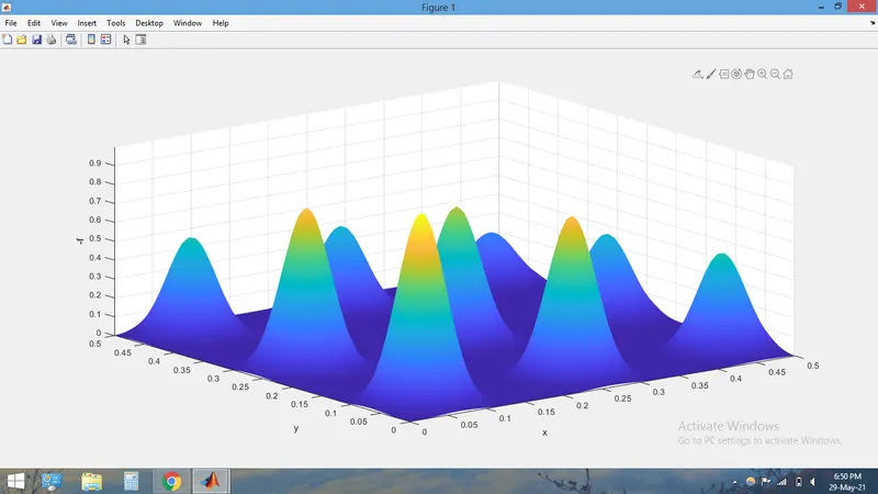
code for the plotting the stalgmite function

clear all
close all
clc

%%plotting the stalagmite function
x=linspace(0,0.5,100);
y=linspace(0,0.5,100);
%creating the two dimensional mesh
[xx yy]=meshgrid(x,y);

for i=1:length(xx)
   %creating the vector input for the stalagmite function
        for j=1:length(yy)
              vector(1)=xx(i,j);
              vector(2)=yy(i,j);
           f(i,j)=stalagmite(vector);
end
              
end 
figure(1)
surfc(x,y,-f)
xlabel('x')
ylabel('y')
zlabel('-f')
shading interp

output of this code

step 2

genetic algorithm for unbounded inputs

%%unbounded inputs
tic             %using tic and toc command for the recording the time
num_cases=20;    %definig the number of times genetic algorithm runs and selects the population size
for i=1:num_cases
[inputs,fval(i)]=ga(@stalagmite,2)
xopt(i)=inputs(1);      %storing the inputs in a different variables for plotting the graph
yopt(i)=inputs(2);
end
study1_time=toc
figure(2)

%subplot for the two plots in the same figure window
subplot(2,1,1)
hold on
surfc(x,y,-f)
xlabel('x')
ylabel('y')
zlabel('f')
plot3(xopt,yopt,-fval,'marker','o') 
title('unbounded inputs')
subplot(2,1,2)
plot(-fval)
xlabel('iteration')
ylabel('function maximum')

explanation of the code

1)tic toc command is used for recording the time of the itetrations

2)number of iterations are defined as 20

3)for loop is introduced for the performing the iteration by 20 times

4)output from the genetic algorithm is stored in the inputs and fval

5)the inputs raw vector was assingn to two different variables and stored as xopt and yopt

6)value of the function is plotted using plot3 for different iteration

7)appropriate legends and labels are given

output of this code

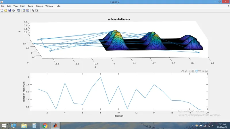
second time i have run the same code

output

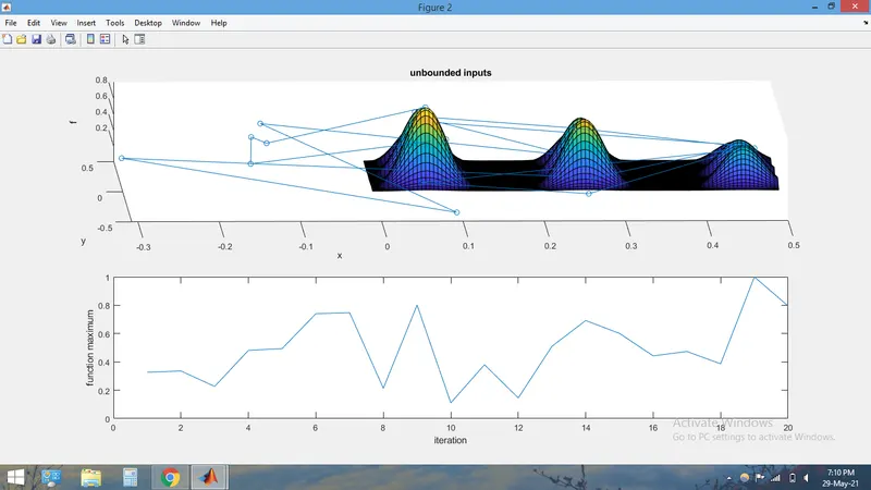
explanation of the output

every time we run this code it is taking the values of x and y from the outside of our domain of the function and gives the maximum values for the function

which is not the correct solution of our problem.so we have to specify our bounds for the x and y values in the genetic algorithm syntax

study time=20.4657seconds

step2)genetic algorithm for the bounded inputs

the only difference here is that the ga code will take values of x and y from the defined inputs.

%%study2 defining the upper and lower bound
tic
num_cases=20;
for i=1:num_cases
[inputs,fval(i)]=ga(@stalagmite,2,[],[],[],[],[0 0],[0.5 0.5]);  %bounding t
xopt(i)=inputs(1);
yopt(i)=inputs(2);
end
study2_time=toc
figure(3)
subplot(2,1,1)
hold on
surfc(x,y,-f)
xlabel('x')
ylabel('y')
zlabel('-f')

plot3(xopt,yopt,-fval,'marker','o') 
title('bounded  inputs')
subplot(2,1,2)
plot(-fval)
xlabel('iteration')
ylabel('function maximum')

output

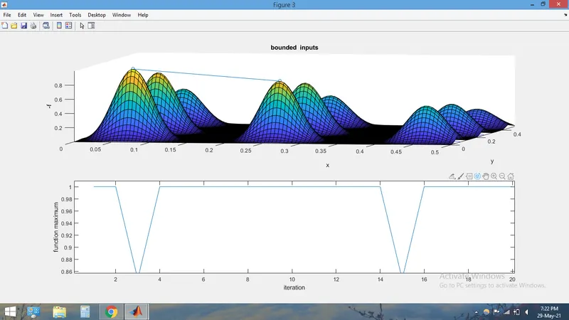
from the output we can see that this code is giving the bounded inputs to the ga it is giving the maximum value for the function for most of the iteration and the value is 1.

study time=37.9426seconds

step3)increasing the population size for the ga by optimoptions and make it 230.

%%study3 defining the upper and lower bound as well as increasing the
%%population size

options=optimoptions('ga');
options=optimoptions(options,'populationsize',230);
tic
num_cases=20;
for i=1:num_cases
[inputs,fval(i)]=ga(@stalagmite,2,[],[],[],[],[0 0],[1 1],[],[],options);
xopt(i)=inputs(1);
yopt(i)=inputs(2);
end
study2_time=toc
figure(4)
subplot(2,1,1)
hold on
surfc(x,y,-f)
xlabel('x')
ylabel('y')
zlabel('f')

shading interp 
plot3(xopt,yopt,-fval,'marker','o') 
title('bounded inputs with increasing population size')
subplot(2,1,2)
plot(-fval)
xlabel('iteration')
ylabel('function maximum')

output

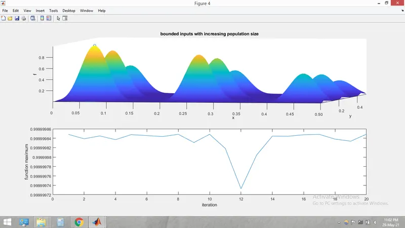
from increasing the population size and defining the upper bound and lower bound we are able to find global maxima for the stalagmite function.

the maximum value is nearly 1 as we can see from the plot.

study time =102.5697seconds

no errors were faced during the coding of this problem.