Week 3.5 - Deriving 4th order approximation of a 2nd order derivative using Taylor Table method

`(d^2f)/(dx^2)=f''(x)`

the number of nodes required for the central difference scheme is=p+q-1

where

p= order of derivative

q= order of approximation

so for the central difference approximation the number of node is =p+q-1

=2+4-1=5

taylor table for the central difference

	f(i)	dx*f'(x)	dx*f''(x)	dx*f'''(x)	dx*fIV(x)	dx*fV(x)
a*f(i-2)	a	-2a	2a	(-8/6)a	(16/24)a	(32/120)a
b*f(i-1)	b	-b	b/2	(-b/6)	b/24	(-b/120)
c*f(i)	c	0	0	0	0	0
d*f(i+1)	d	d	d/2	d/6	d/24	d/120
e*f(i+2)	e	2e	2e	(8/6)e	(2/3)e	(32/120)e
sum of terms d2f/dx2	0	0	1	0	0	0

by the taylor table we can derove following equations

a+b+c+d+e=0

-2a-b+d+2e=0

2a+b/2+d/2+2e=1

-(8/6)a-(b/6)+d/6+(8/6)e=0

(16/24)a+(b/24)+(d/24)+(2/3)e=0

we have 5 unknowns and 5 equations so we can find out the value of unknown

writing the above equation in matrix form

by solving above equation in matlab using linsolve command we get

a=-0.0833,b=1.3333,c=-2.5000,d=1.3333,e=-0.0833

substituting the values

`(d^2f)/(dx^2)=[a*f(i-2)+b*f(i-1)+c*f(i)+d*f(i+1)+e*f(i+2)]/(dx^2)`

`(d^2f)/(dx^2)=[-0.0833*f(i-2)+1.3333*f(i-1)-2.5f(i)+1.3333*f(i+1)-0.0833*f(i+2))]/(dx^2))`

The number of nodes required for the skewed right sided scheme

=p+q=2+4=6

Taylor table 4^th order approximation of second derivative forward difference

	F(x)	F’(x)dx	F’’(x)(dx^2)	F’’’(x)(dx^3)	FIV(x)(dx^4)	FV(x)(dx^5)	FVI(x)(dx^6)
hf(i)	h	0	0	0	0	0	0
jf(i+1)	j	J	j(1/2)	j(1/6)	j(1/24)	j(1/120)	j/720
kf(i+2)	k	k(2)	k(4/2)	k(8/6)	k(16/24)	k(32/120)	(64/720)k
lf(i+3)	l	3l	l(9/2)	l(27/6)	l(81/24)	l(243/120)	(729/720)l
mf(i+4)	m	4m	m(16/2)	m(64/6)	m(256/24)	m(1024/120)	(4096/720)m
nf(i+5)	n	5n	n(25/2)	n(125/6)	n(625/24)	n(3125/120)	(15625/720)n
Sum of above terms d2f/dX2	0	0	1	0	0	0	Don’t know

The equation from the above taylor table

h+j+k+l+m+n=0

j+2k+3l+4m+5n=0

j(1/2)+ k(4/2)+ l(9/2)+ m(16/2)+ n(25/2)=1

j(1/6)+ k(8/6)+ l(27/6)+ m(64/6)+ n(125/6)=0

j(1/24)+ k(16/24)+ l(81/24)+ m(256/24)+ n(625/24)=0

j(1/120)+(32/120)k+(243/120)l+(1024/120)m+(3125/120)n=0

by solving this equations in matlab using the linsolve command

h=3.7500,

j= -12.8333,

k=17.8333,

l= -13,

m=5.088,

n= -0.8333

`(d^2f)/(dx^2)=[3.7500*f(i)-12.8333*f(i+1)+17.8333*f(i+2)-13*f(i+3)+5.088*f(i+4)-0.08333 f(i+5))]/(dx^2))`

Taylor table 4^th order approximation of second derivative using backward difference

The number of nodes required for the skewed right sided scheme

=p+q=2+4=6

	F(x)	F’(x)dx	F’’(x)(dx^2)	F’’’(x)(dx^3)	FIV(x)(dx^4)	FV(x)(dx^5)	FVI(x)(dx^6)
pf(i-5)	P	-5p	p(25/2)	-p(25/6)	p(625/24)	-p(3125/120)	(15625/720)p
qf(i-4)	Q	-4q	q(16/2)	-q(64/6)	q(256/24)	-q(1024/120)	(4096/720)q
rf(i-3)	R	-3r	r(9/2)	-r(27/6)	r(81/24)	-r(243/120)	(729/720)r
sf(i-2)	S	-s(2)	s(4/2)	-s(8/6)	s(16/24)	-s(32/120)	(64/720)s
tf(i-1)	t	-t	t(1/2)	-t(1/6)	t(1/24)	-t(1/120)	t/720
uf(i)	u	0	0	0	0	0	0
Sum of above terms d2f/dX2	0	0	1	0	0	0	Don’t know

From the taylor table we can get this equations

p+q+r+s+t+u=0

-t-2s-3r-4q-5p=0

t(1/2)+ s(4/2)+ r(9/2)+ q(16/2)+ p(25/2)=1

-t(1/6)- s(8/6)- r(27/6)- q(64/6)- p(125/6)=0

t(1/24)+ s(16/24)+ r(81/24)+ q(256/24)+ p(625/24)=0

-t(1/120)-(32/120)s-(243/120)r-(1024/120)q-(3125/120)p=0

By solving the above equation we get

u=3.7500,

t= -12.8333,

s= 17.8333,

r= -13.0000,

q= 5.0833,

p= -0.8333

`(d^2f)/(dx^2)=[-0.8333*f(i-5)+5.0833*f(i-4)-13*f(i-3)+17.8333*f(i-2)-12.8333*f(i-1)+3.7500 *f(i))]/(dx^2))`

matlab code for the fourth order approximation of second order derivative

clear all
close all
clc
%fourth order approximation  of second order dervative  using taylor table
x=pi/3;
dx=linspace(pi/4000,pi/40,20);     %defining the range of dx

%% solving the second derivative of function exp(x)*cos(x)
%analytical derivative=-2*exp(x)*sin(x)
analytical_derivative=-2*exp(x)*sin(x);
 
%numerical derivative 

%% fourth order approximation by central difference 
%creating the matrix by taylor table 
A=[1 1 1 1 1;-2 -1 0 1 2;4/2 1/2 0 1/2 4/2;-8/6 -1/6 0 1/6 8/6;2/3 1/24 0 1/24 2/3];
B=[0;0;1;0;0];
X=inv(A)*B;            %solving the matrix
a=X(1);                 %deriving the value of coefficient
b=X(2)
c=X(3);
d=X(4);
e=X(5);


%calling the function cdasfun(central difference approxomation scheme)
for i=1:length(dx)
    
    c_d_a_s(i)=cdasfun(x,dx(i),a,b,c,d,e)
    cdaserror(i)=abs(c_d_a_s(i)-analytical_derivative)
end
loglog(dx,cdaserror,'color','r') 
hold on

%%fourth order approximation by skewed forward difference
%creating the matrix by taylor table
P=[1,1,1,1,1,1;0,1,2,3,4,5;0,1/2,4/2,9/2,16/2,25/2;0,1/6,8/6,27/6,64/6,125/6;0,1/24,16/24,81/24,256/24,625/24;0,1/120,32/120,243/120,1024/120,3125/120];
Q=[0;0;1;0;0;0];
R=inv(P)*Q;
h=R(1);
j=R(2);
k=R(3);
l=R(4);
m=R(5);
n=R(6);
%calling the function fdasfun(forward difference approxomation scheme)

for i=1:length(dx)
    
    f_d_a_s(i)=fdasfun(x,dx(i),h,j,k,l,m,n)
    fdaserror(i)=abs(f_d_a_s(i)-analytical_derivative)
end
loglog(dx,fdaserror,'color','b')  
hold on


%%fourth order approximation by skewed BACKWARD difference
%creating the matrix by taylor table
M=[1,1,1,1,1,1;-5,-4,-3,-2,-1,0;25/2,16/2,9/2,4/2,1/2,0;-125/6,-64/6,-27/6,-8/6,-1/6,0;625/24,256/24,81/24,16/24,1/24,0;-3125/120,-1024/120,-243/120,-32/120,-1/120,0]
N=[0;0;1;0;0;0];
O=inv(M)*N;
p=O(1);
q=O(2);
r=O(3);
s=O(4);
t=O(5);
u=O(6);
%calling the function bdasfun(backward difference approxomation scheme)

for i=1:length(dx)
    
    b_d_a_s(i)=bdasfun(x,dx(i),p,q,r,s,t,u)
    bdaserror(i)=abs(b_d_a_s(i)-analytical_derivative)
end
loglog(dx,bdaserror,'color','g')  
hold on
legend('cdas error','fdas error','bdas error')
xlabel('dx')
ylabel('errors')

cdasfun code

function c_d_a_s=cdasfun(x,dx,a,b,c,d,e)

c_d_a_s=[a*exp(x-2*dx)*cos(x-2*dx)+b*exp(x-dx)*cos(x-dx)+c*exp(x)*cos(x)+d*exp(x+dx)*cos(x+dx)+e*exp(x+2*dx)*cos(x+2*dx)]/(dx^2)
%cdaserror=abs(c_d_a_s-analytical_derivative);
end

fdasfun code

function f_d_a_s=fdasfun(x,dx,h,j,k,l,m,n)

f_d_a_s=[h*exp(x)*cos(x)+j*exp(x+dx)*cos(x+dx)+k*exp(x+2*dx)*cos(x+2*dx)+l*exp(x+3*dx)*cos(x+3*dx)+m*exp(x+4*dx)*cos(x+4*dx)+n*exp(x+5*dx)*cos(x+5*dx)]/(dx^2)

end

bdasfun code

function b_d_a_s=bdasfun(x,dx,p,q,r,s,t,u)
b_d_a_s=[p*exp(x-5*dx)*cos(x-5*dx)+q*exp(x-4*dx)*cos(x-4*dx)+r*exp(x-3*dx)*cos(x-3*dx)+s*exp(x-2*dx)*cos(x-2*dx)+t*exp(x-dx)*cos(x-dx)+u*exp(x)*cos(x)]/(dx^2)


end

Step wise explanation of the code

1)by clear all close all and clc we cleared any previous variables aswell as the plots

2)writing the programe by starting with the comment

3)defining the value of x at which we want to find out the second order derivative

]4)the Range of the dx is defined by the linspace command

5)finding the value of the analytical derivative

Finding the numerical derivative by forward difference scheme

6)finding the vector X which is the solution vector for the central difference approximation by inverse of matix A.

7)introducing the for loop for taking the value of dx for calculating the value of central difference approximation and calculating the error.

8)plotting the loglog graph for the dx vs cdsa error

Finding the numerical derivative by backward difference scheme

9)finding the vector R which is the solution vector for the forward difference approximation by inverse of matix P.

10)introducing the for loop for taking the value of dx for calculating the value of forward difference approximation and calculating the error.

11)plotting the loglog graph for the dx vs fdsa error

12)finding the vector O which is the solution vector for the backward difference approximation by inverse of matix M.

13)introducing the for loop for taking the value of dx for calculating the value of backward difference approximation and calculating the error.

14)plotting the loglog graph for the dx vs bdsa error

output plot

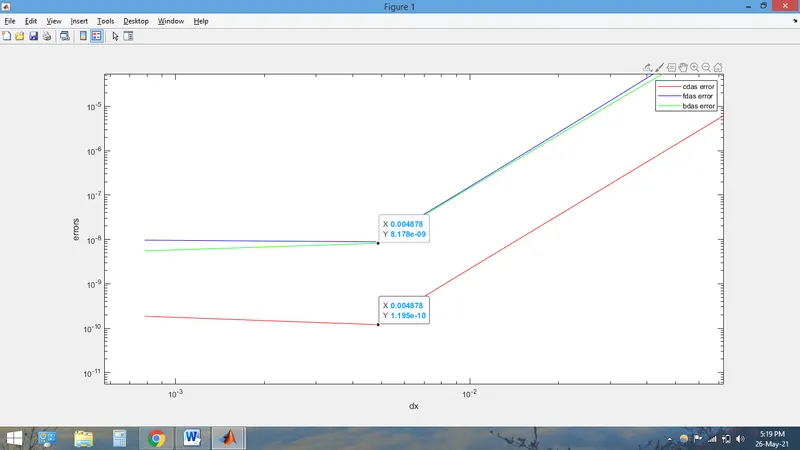
from the plot of different errors vs the dx we can see that the lowest value for the error is for the central difference approximation scheme

by increasing the value of dx after the 0.004878 the value of all the errors is increasing

by decreasing the value of dx after the 0.004878 the errors also starts to increase due to round of errors in the debugging of the code