Week 8- Moving zones approach in Fluent
1.What are the approaches by which you would model moving zones?
Moving Reference Frame (MRF)
The MRF model is the simplest of the two approaches for multiple zones. It is a steady-state approximation in which individual cell zones move at different rotational and/or translational speeds. The flow in each moving cell zone is solved using the moving reference frame equations. If the zone is stationary {tex}(\omega = 0){/tex}, the stationary equations are used i.e., moving reference frame equations are solved in rotational zone and stationary equations are solved in stationary zone and the information is exchanged at the interface. The properties of the flow at the interface between the stationary and rotating zones is directly translated in MRF. In MRF approach there is no relative motion between moving zone with respect to the adjacent zone, the grid is fixed for computation. This is analogous to freezing the motion of the moving part in a specific position and observing the instantaneous flow field with the rotor in that position and hence, the MRF is often referred to the "frozen rotor approach."
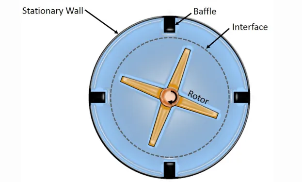
An example that illustrates the MRF approach is shown with an above (image). In the image apart from the rotor and stationary walls there are stationary baffles present inside the fluid zone. Thus an interface is defined which is a surface of revolution about the rotor axis to distinguish between stationary and rotating zone. MRF model should be used when the flow is not complicated and if the interaction between rotor and stator in a turbine stage is weak. With a MRF simulation rotating wakes, secondary flows, leading edge pressure increases etc.will always stay in exactly the same positions. This makes the simulation very dependent on exactly how the rotors and the stators are positioned. Usually MRF model is used to calculate flow field that can be used as initial condition for sliding mesh calculation.
Moving Mesh Method (MMM)
In moving mesh methods, physical PDEs and a mesh equation derived from equidistribution of an error metrics (so-called the monitor function) are simultaneously solved and meshes are dynamically concentrated on steep regions
2.Which approach would you use to model unsteady phenomena?
Sliding moving mesh method
In a time-accurate solution for rotor-stator interaction (rather than a time-averaged solution) is desired, you must use the sliding mesh model to compute the unsteady flow field. The sliding mesh model is the most accurate method for simulating flows in multiple moving reference frames and is the most computationally demanding. As was mentioned, the sliding mesh model is theoretically the most accurate method for simulating rotating flows, and it can correctly describe the whole transient startup. However, it is also the most computationally demanding. This technique, applied to the specific case, results in two cell zones created separately. Each cell zone is bounded by an interface that meets the opposing cell zone. The two cell zones will slide relative to one another along the mesh interface in discrete steps.
3.Procedure
a.The mesh was directly copied into ANSYS-Fluent.
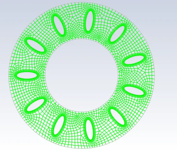
b. The RPM is set to 250.
c.The fluid used here as reference is air.
d.Viscous model used here is K-Epsilon realizable.
c.The iterations are done upto 1000.
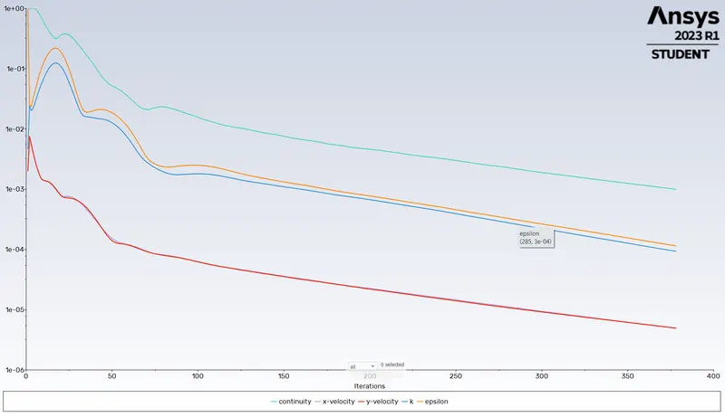
d.The maximum velocity attained here is 23m/s.
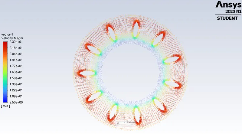
Result
The simulation for the rotary motion for the geometry is done and the velocity profile for the fluid motion is plotted.