Week 8- Moving zones approach in Fluent

Aim

To simulate a rotary motion of fluid for the given geometry and plot the velocity profile.

Introduction

Moving zones in fluid flows can be in the form of linear or rotary motions. Modeling these moving zones can be done in two methods:

1. Moving Reference Frame Method
   
   This method is a steady-state approximation of the motion of the moving zone at a particular instant of time. This method does not require changing the mesh and does not take into account the transient behavior of the flow making it computationally cheaper. The governing equations are modified using the moving frame of reference compared to the stationary zones in the domain. This flow simplification when used appropriately will provide good approximations of the transient moving zones' behavior in the fluid with minimal computational cost.
2. Moving Mesh Method
   
   This method involves a fully unsteady simulation where the mesh and domain are altered across each timestep based on the motion of the moving zones. This method is computationally expensive and is performed when the transient behavior of the fluid is of importance. A mesh interface is generated between the stationary and moving parts of the mesh where interpolation of the quantities is conducted (when the mesh is non-conformal) to ensure seamless movement of the fluid zone.

Unsteady flow phenomena can be modeled using the moving mesh method as it varies the mesh and domain at each time step corresponding to the motion of the moving zone.

Method

Domain and Mesh

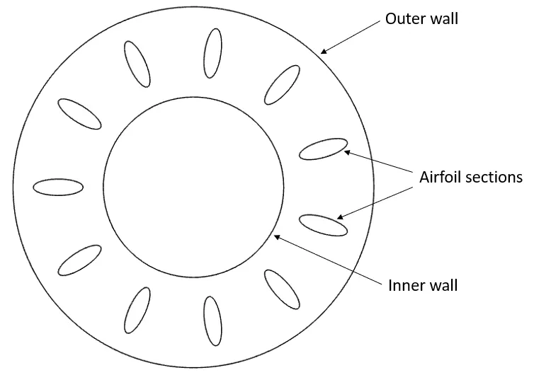
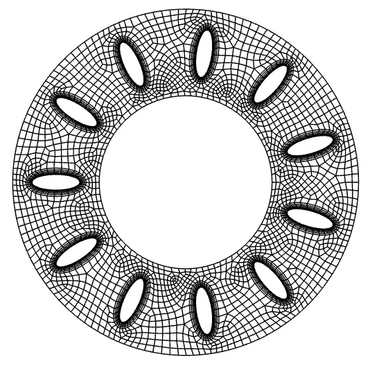
The domain and mesh were provided and shown in the image below.

CFD Setup

The simulation was conducted on ANSYS Fluent 2022R2. Air was used as the fluid with default properties. The fluid zone was set to a rotary moving frame of reference with an rpm of 250 with the axis of rotation at the center of the domain. The airfoils were set to a moving wall with motion set relative to the adjacent cell zone.

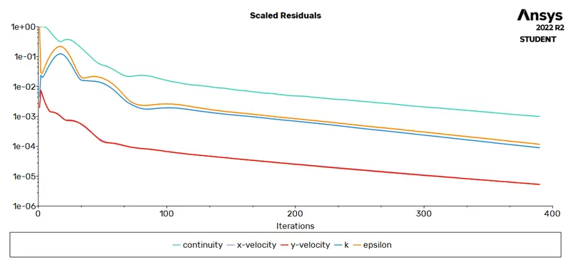
The steady-state pressure-based PV coupled solver was used to discretize the flow parameters. Turbulence in the flow was predicted using the two-equation Realizable K-Epsilon model with enhanced wall treatment. The second-order scheme was used to estimate the pressure, the second-order upwind scheme was used to estimate momentum and turbulence parameters. The solution was initialized by a hybrid initialization. The simulation was run with pseudo transient time stepping with an automatic global conservative length scale. Convergence was checked by scaled residuals achieving 1e-3 units and the simulation converged within 400 iterations.

Results

The image below shows the scaled residuals to ensure convergence of the simulation.

The images below show the velocity distribution and velocity vectors in the domain.

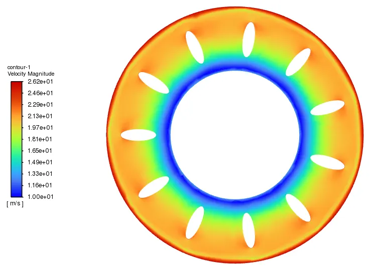
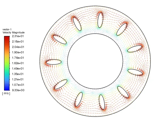
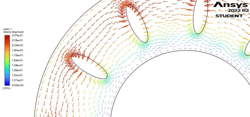
The velocity distribution profiles show that the high-velocity flow is present near the outer wall of the domain and the low-velocity flow is present near the inner wall. Acceleration of the flow can be seen on either side of the airfoil.

Conclusion

The rotational motion of the fluid was simulated using the moving frame of reference method on the given mesh. The velocity profiles were plotted and showed increased velocities near the outer wall of the domain and decreased velocities near the inner walls. An acceleration of the flow was also observed at either end of each airfoil section.