Moving zones approach in Fluent

In today’s topic, we will discuss about moving zones. Before discussing this phenomenon, one must first understand why do we need it.

All the models and setups discussed earlier had stationary objects under study. Hence, the mesh around it was also stationary. But, not every study/case has stationary objects. In fact, most of the industrial applications have moving components. Using a normal approach for such studies would give us absurd results. This is because a moving component would also distort the mesh around it and hence improper transfer of quantities over the mesh would take place.

Numerous methods have been developed over the years to overcome this problem. With time, additional features have been added in the tools to make these methods as accurate as the real-world solutions.

The motion of the moving objects can be either classified as rectilinear or rotary (There are other motions like Simple Harmonic Motion and much more complex motions). Today’s discussion would be limited for Rotary motion only.

There are two approaches for solving rotatory motions.

1. Moving Reference Frame (MRF) approach
2. Moving Zones approach

1. Moving Reference Frame (MRF)

In this approach, we segregate the domain based on the behavior of components in them. For example, the domain where the components are moving/rotating and the domain around them where the motion of the components have significant effect on the fluid is assigned as one zone. And the rest as other or as required.

In this approach, the Mesh is stationary and it doesn’t change with respect to time/computations. Rather an additional term/equation is added into the N-S equation to simulate the Rotatory motion. These equations are solved only in the region which is defined as moving by the user.

In this case, we are basically solving the problem from the reference of the moving frame rather than the inertial frame. This makes the problem steady in nature.

This approach is particularly useful when dealing with Steady flows or studies where unsteadiness is not important.

The non-inertial frame and inertial frames are segregated by an interface. The data transfer at this interface can happen in 3-possible ways.

1. Area averaging
2. Mass averaging
3. Mixed-out approach.

The Mixed-out approach is the most accurate one, as it solves the governing equations at the interface and transfers data accordingly.

MRF is further classified as Single Reference Frame approach and Multiple Reference Frame approach.

2. Moving – Mesh approach

In this approach the mesh changes with respect to time, it changes as per motion of the moving component. To avoid skewed or negative volume elements different methods are employed. This increases the number of calculations which happen at every iteration. Thus, making the simulation extremely expensive when compared to the MRF approach.

This approach is employed for Un-steady flows. But it can also solve Steady flows. The solution of the MRF approach is used as the initial condition for the Moving – Mesh approach.

Simulation of Rotary Motion

1. Import the geometry
2. Steady state & pressure based
3. Viscous model- K-Omega - Realizable with Enhanced wall treatment
4. Cell zone condition - Frame motion with 250 rpm
5. Boundary conditions - Airfoil - Moving wall relative to adjacent cell zone with rotational motion
6. Method - Coupled second order
7. Control - Couranth number - 10

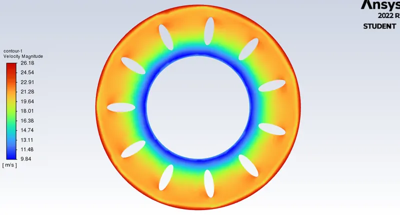
Conclusion

As we move farther from the center, the velocity is increases. Also, there is a small region of high velocity at the blade tips.