Simulating a Laminar Flow through a pipe using OpenFoam
In this project, A laminar incompressible fluid flow through a cylindrical pipe is simulated using OpenFoam and is validated using Analytical results obtained from MATLAB.
Hagen-Poiseullie's law
The Laminar incompressible flow is governed by Hagen-Poiseullie's law. It gives the pressure drop in a Laminar incompressible and Newtonian fluid flowing through a long cylindrical pipe of constant cross-section.
Assumptions
- Laminar flow - A flow is said to be laminar if the fluid layers run smoothly over each other and do not intermix. In mathematical terms, a flow whose Reynolds number is less than a specified value (which varies from situation to situation) is a Laminar flow.
To understand more about the flow behaviour, I strongly recommend you to watch this video by "The Efficient Engineer". - Incompressible flow - A flow is said to be incompressible if it doesn't compress under pressure, in mathematical terms, its density remains constant throughout the flow.
- Newtonian fluid - A Newtonian fluid is a fluid in which the viscous stresses arising from the flow are, at every point linearly correlated to the local strain rate.
`tau alpha (delu)/(dely)`
`tau = mu(delu)/(dely)` - Dimensional Constraints - The length of the pipe should be substantially longer than its diameter.
`l/r<(Re)/48`
where,
l is the length of the pipe
r is the radius of the pipe, and
Re is the Reynolds number of the flow.
Mathematical Equation
`Deltap=(8mulQ)/(pir^4)`
where,
`Deltap` is the pressure drop across the pipe
`mu` is the dynamic viscosity
`l` is the length of the pipe
`Q` is the volumetric flow rate, and
`r` is the radius of the pipe.
The derivation to the above equation can be found in any standard Fluid dynamics textbook.
Applications
- Airflow in lung alveoli
- Flow-through a drinking straw
- Flow-through a hypodermic needle
Introduction to Darcy-Weisbach equation
The pressure drop calculated from Hagen-Poiseullie's law is related to the wall shear stress, which is obtained from the Darcy-Weisbach equation. In the case of Laminar flow for a circular cross-section, the co-relation is as shown below
`Lambda = 64/(Re)`
where,
`Lambda` is the shear stress, and
`Re`, as defined earlier, is the Reynolds number.
`(Deltap)/L=Lambdarhov^2/(2d)`
where,
`Deltap` is the pressure drop due to viscous effects.
`rho` is the density of the flow
`v` is the mean flow velocity, and
`d` is the diameter of the pipe.
Laminar flow through a pipe of uniform circular cross-section
If there were no viscosity and friction, the flow properties might remain constant throughout the pipe; but that is not how it works. In real-world situations, we have viscosity, friction and tons of other stuff like capillarity, surface tension, and cavitation, which are too complex to take into account in a single problem.
When the flow enters a pipe, it comes into contact with its cross-section. Since the walls are stationary, they would slow down the fluid and that is what happens, but only partially. The flow slows down only near the walls and surprisingly it speeds up at the centre, it almost doubles to what it was initially. Before the flow develops fully ( Steady state ), it goes through different stages ( Transient state ). The velocity profile's for these are shown in the above picture.
Hydrodynamic Region is the distance the fluid has to travel before reaching the fully developed region. For Laminar flow, it is given by the equation
`L_H = 0.057dRe`
Parameters used
Density is assumed as 1 (since it is inbuilt in OpenFoam, also the flow is incompressible), Reynolds number as 2100 (Laminar Flow, Re<2400), kinematic viscosity as 0.01 (random), diameter as 1m (random). From these conditions, velocity can be found as 21m/s and length should be greater than 21.874 m. Hydrodynamic distance is calculated to be 119.7, So to obtain a developed flow, the length should be greater than 120 m. We choose the length to be 200m.
Step 1: Solver Selection
OpenFoam documentation [4] is the best to decide which solver can be useful for a specific application. Since the flow in focus is Laminar, Newtonian and incompressible in nature, icoFoam would be an ideal choice.
Copy the necessary tut from the tut folder, paste it into the run folder and work on it here.
Step 2: Geometry and Mesh Generation
For this project, we are creating Geometry and generating Mesh using the blockMeshDict file, which is an inbuilt file in all the solvers.
Some Mesh types that can be used ( not exhaustive )
Case 1: Axi-Symmetric wedge
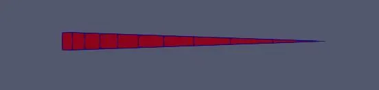
In this case, we generate an axisymmetric wedge i.e we create a geometry of a wedge, Mesh it and run the solver on it. The boundary conditions are given as such, that it is equal to simulating a flow in a full cylinder/pipe.
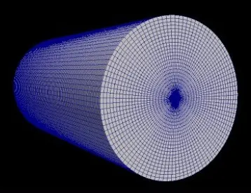
It can be seen that the Mesh is very fine at the centre of the cylinder, but coarse at the boundary. This looks good visually but doesn't make any sense, because, in reality, most of the action takes place at the boundary, where the wall shear stress is present. So there is a good chance that the solution might converge, but might not be very accurate.
Case 2 :
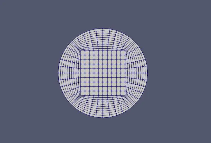
Here, the Mesh is finer at the boundaries than the centre. This solves the problem faced in Case 1. We can make this Mesh further better, by removing the abrupt change from square meshes to angular meshes.
Case 3 :
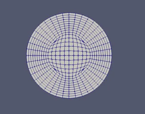
Here, the Mesh is concentrated at boundaries, and the transition is also smooth. So this is the winner of the three cases. But in this project we use Case 1 because it takes far less computation time, thus Money, when compared to the other 2 cases. This is because the solver is acting only on the wedge.
This is the trade-off every CFD engineer has to decide on, more accuracy ? or less expensive? The solution lies in the type of problem at hand.
However, I will provide the blockMeshDict file for this case at the end and you can run it on your PC. If you have any Meshes which can give better results than the ones mentioned above, please feel free to describe/show them in the comments section.
Geometry and Mesh generation for Case 1
path : run>cavity>cavity>system>blockMeshDict
To make things a bit lengthy, we are using MATLAB to create a blockMeshDict file, instead of directly editing it in the terminal.
Here is the MATLAB code for it :
clear all
close all
clc

b=fopen('blockMeshDict.txt','w')

fprintf(b,'FoamFilen')
fprintf(b,'{n')
fprintf(b,'    format      ascii;n')
fprintf(b,'    class       dictionary;n')
fprintf(b,'    object      blockMeshDict;n')
fprintf(b,'}n')
fprintf(b,'convertToMeters 1;n')
display('(l/r)>(R_e/48)n')
display('Reynolds number = 2100')
Re=2100;
r=input('The radius of pipe is ')
l=input('Length of pipe is ')
theta=input('Wedge angle is ')
fprintf(b,'r %f;n',r)
fprintf(b,'l %f;n',l)
fprintf(b,'theta %f;n',theta)
fprintf(b,'ct #calc "cos(degToRad($theta))";n')
fprintf(b,'st #calc "sin(degToRad($theta))";n')
fprintf(b,'nct #calc "cos(degToRad(-$theta))";n')
fprintf(b,'nst #calc "sin(degToRad(-$theta))";n')
fprintf(b,'rct #calc "$r*$ct";n')
fprintf(b,'rst #calc "$r*$st";n')
fprintf(b,'nrct #calc "$r*$nct";n')
fprintf(b,'nrst #calc "$r*$nst";n')
fprintf(b,'verticesn')
fprintf(b,'(n')
fprintf(b,'    (0 0 0)		//0n')
fprintf(b,'    (0 $nrct $nrst)	//1n')
fprintf(b,'    (0 $rct $rst)	//2n')
fprintf(b,'    ($l 0 0)		//3n')
fprintf(b,'    ($l $nrct $nrst)	//4n')
fprintf(b,'    ($l $rct $rst)	//5n')
fprintf(b,');n')
fprintf(b,'blocksn')
fprintf(b,'(n')
fprintf(b,'    hex (1 4 5 2 0 3 3 0) (400 1 10) simpleGrading (1 1 5)n')
fprintf(b,');n')
fprintf(b,'edgesn')
fprintf(b,'(n')
fprintf(b,'    arc 1 2 (0 $r 0)n')
fprintf(b,'    arc 4 5 ($l $r 0)n')
fprintf(b,');n')
fprintf(b,'boundaryn')
fprintf(b,'(n')
fprintf(b,'    inletn')
fprintf(b,'    {n')
fprintf(b,'        type patch;n')
fprintf(b,'        facesn')
fprintf(b,'        (n')
fprintf(b,'            (0 1 2 0)n')
fprintf(b,'        );n')
fprintf(b,'    }n')
fprintf(b,'    outletn')
fprintf(b,'    {n')
fprintf(b,'        type patch;n')
fprintf(b,'        facesn')
fprintf(b,'        (n')
fprintf(b,'            (3 5 4 3)n')
fprintf(b,'        );n')
fprintf(b,'    }n')
fprintf(b,'    bottomsiden')
fprintf(b,'    {n')
fprintf(b,'        type wedge;n')
fprintf(b,'        facesn')
fprintf(b,'        (n')
fprintf(b,'            (0 3 4 1)n')
fprintf(b,'        );n')
fprintf(b,'    }n')
fprintf(b,'    topsiden')
fprintf(b,'    {n')
fprintf(b,'        type wedge;n')
fprintf(b,'        facesn')
fprintf(b,'        (n')
fprintf(b,'            (0 2 5 3)n')
fprintf(b,'        );n')
fprintf(b,'    }n')
fprintf(b,'    fixedWallsn')
fprintf(b,'    {n')
fprintf(b,'        type wall;n')
fprintf(b,'        facesn')
fprintf(b,'        (n')
fprintf(b,'            (1 4 5 2)n')
fprintf(b,'        );n')
fprintf(b,'    }n')
fprintf(b,'    axisn')
fprintf(b,'    {n')
fprintf(b,'    	type empty;n')
fprintf(b,'    	facesn')
fprintf(b,'    	(n')
fprintf(b,'    	    (0 3 3 0)n')
fprintf(b,'    	);n')
fprintf(b,'    }n')
fprintf(b,');n')
fprintf(b,'mergePatchPairsn')
fprintf(b,'(n')
fprintf(b,');n')
fclose(b)
Explanation of the code used above - Simple file generating, and writing commands have been used, and the lines printed are written in a way to match with the actual blockMeshDict files, this is because the terminal window in OpenFoam uses C++ language, which, unlike MATLAB, cares about the indentations and would throw an error if wrongly indented.
Inputs provided
Radius of pipe = 0.5 m
Length of pipe = 200m
Wedge Angle = 2degrees
Output -
FoamFile
{
    format      ascii;
    class       dictionary;
    object      blockMeshDict;
}
convertToMeters 1;
r 0.500000;
l 200.000000;
theta 2.000000;
ct #calc "cos(degToRad($theta))";
st #calc "sin(degToRad($theta))";
nct #calc "cos(degToRad(-$theta))";
nst #calc "sin(degToRad(-$theta))";
rct #calc "$r*$ct";
rst #calc "$r*$st";
nrct #calc "$r*$nct";
nrst #calc "$r*$nst";
vertices
(
    (0 0 0)		//0
    (0 $nrct $nrst)	//1
    (0 $rct $rst)	//2
    ($l 0 0)		//3
    ($l $nrct $nrst)	//4
    ($l $rct $rst)	//5
);
blocks
(
    hex (1 4 5 2 0 3 3 0) (400 1 10) simpleGrading (1 1 5)
);
edges
(
    arc 1 2 (0 $r 0)
    arc 4 5 ($l $r 0)
);
boundary
(
    inlet
    {
        type patch;
        faces
        (
            (0 1 2 0)
        );
    }
    outlet
    {
        type patch;
        faces
        (
            (3 5 4 3)
        );
    }
    bottomside
    {
        type wedge;
        faces
        (
            (0 3 4 1)
        );
    }
    topside
    {
        type wedge;
        faces
        (
            (0 2 5 3)
        );
    }
    fixedWalls
    {
        type wall;
        faces
        (
            (1 4 5 2)
        );
    }
    axis
    {
    	type empty;
    	faces
    	(
    	    (0 3 3 0)
    	);
    }
);
mergePatchPairs
(
);
Replace the actual blockMeshDict file of the solver with the file generated above and run the blockMesh Command. (OpenFoam might throw an error regarding the file format, which means OpenFoam can not run the .txt file and you will need to find a method to overcome this)
Run blockMesh, open paraFoam and verify if the Geometry generated is correct.
Step 3: Update the Initial conditions, Boundary conditions and Constants
3.1 - Pressure
Pressure conditions are specified at all the relevant boundaries.
/*--------------------------------*- C++ -*----------------------------------*
  =========                 |
  \      /  F ield         | OpenFOAM: The Open Source CFD Toolbox
   \    /   O peration     | Website:  https://openfoam.org
    \  /    A nd           | Version:  9
     \/     M anipulation  |
*---------------------------------------------------------------------------*/
FoamFile
{
    format      ascii;
    class       volScalarField;
    object      p;
}
// * * * * * * * * * * * * * * * * * * * * * * * * * * * * * * * * * * * * * //

dimensions      [0 2 -2 0 0 0 0];

internalField   uniform 0;

boundaryField
{
    inlet
    {
        type            zeroGradient;
    }

    outlet
    {
        type            fixedValue;
        value		uniform 0;
    }
    bottomside
    {
        type 		wedge;
    }
    topside
    {
        type 		wedge;
    }
    fixedWalls
    {
        type 		zeroGradient;
    }
    axis
    {
    	type 		empty;
    }

}

// ************************************************************************* //
3.2 - Velocity
Velocity, if any, is specified at all the relevant boundaries.
/*--------------------------------*- C++ -*----------------------------------*
  =========                 |
  \      /  F ield         | OpenFOAM: The Open Source CFD Toolbox
   \    /   O peration     | Website:  https://openfoam.org
    \  /    A nd           | Version:  9
     \/     M anipulation  |
*---------------------------------------------------------------------------*/
FoamFile
{
    format      ascii;
    class       volVectorField;
    object      U;
}
// * * * * * * * * * * * * * * * * * * * * * * * * * * * * * * * * * * * * * //

dimensions      [0 1 -1 0 0 0 0];

internalField   uniform (0 0 0);

boundaryField
{
    inlet
    {
        type            fixedValue;
        value           uniform (21 0 0);
    }
    outlet
    {
        type            zeroGradient;

    }
    bottomside
    {
        type 		wedge;
    }
    topside
    {
        type 		wedge;
    }
    fixedWalls
    {
        type 		noSlip;
    }
    axis
    {
    	type 		empty;
    }
}

// ************************************************************************* //
3.3 - Transport properties
Kinematic Viscosity is specified here, in this case, it is 0.01.
/*--------------------------------*- C++ -*----------------------------------*
  =========                 |
  \      /  F ield         | OpenFOAM: The Open Source CFD Toolbox
   \    /   O peration     | Website:  https://openfoam.org
    \  /    A nd           | Version:  9
     \/     M anipulation  |
*---------------------------------------------------------------------------*/
FoamFile
{
    format      ascii;
    class       dictionary;
    location    "constant";
    object      transportProperties;
}
// * * * * * * * * * * * * * * * * * * * * * * * * * * * * * * * * * * * * * //

nu              [0 2 -1 0 0 0 0] 0.01;


// ************************************************************************* //
3.4 - ControlDict
Parameters like run time, start time, end time, timestep etc.. are edited here.
/*--------------------------------*- C++ -*----------------------------------*
  =========                 |
  \      /  F ield         | OpenFOAM: The Open Source CFD Toolbox
   \    /   O peration     | Website:  https://openfoam.org
    \  /    A nd           | Version:  9
     \/     M anipulation  |
*---------------------------------------------------------------------------*/
FoamFile
{
    format      ascii;
    class       dictionary;
    location    "system";
    object      controlDict;
}
// * * * * * * * * * * * * * * * * * * * * * * * * * * * * * * * * * * * * * //

application     icoFoam;

startFrom       startTime;

startTime       0;

stopAt          endTime;

endTime         10;

deltaT          0.01;

writeControl    runTime;

writeInterval   0.1;

purgeWrite      0;

writeFormat     ascii;

writePrecision  6;

writeCompression off;

timeFormat      general;

timePrecision   6;

runTimeModifiable true;


// ************************************************************************* //
3.5 Run the solver
icoFoam is the solver to be used. The obtained results can be visualised in ParaView using the paraFoam command.
Analytical Solution
Re=2100;
r=input('The radius of pipe is ')
l=input('Length of pipe is ')
rho=1;          %incompressible flow
mu=0.01;
d=2*r;
L_H=0.058*Re*d;
v_avg=(Re*mu)/(rho);
r_location=linspace(0,r,10);
v_r=2*v_avg*(1-(r_location./r).^2);

l_location=linspace(0,l,400);

p_drop=(32*mu.*l_location*v_avg)./(d*d);
p_drop=p_drop(end)-p_drop;
darcy_factor=64/Re;
shear_stress=(darcy_factor*0.25*rho*v_avg*v_avg*0.5);

figure(1)

plot(v_r,r_location)
xlabel('Radial Veloctiy')
ylabel('Radial Location')
legend('Analytical solution')

figure(2)
plot(l_location(280:400),p_drop(280:400))
xlabel('Axial Location')
xlim([140 200])
ylabel('Pressure drop')
legend('Analytical Solution')
Results
1. Velocity variation near inlet area and outlet area w.r.t timestep
Above are two different gif files showing the inlet and outlet areas of the pipe. The pipe is too long to fit in a single picture, hence two gifs are used.
It can be seen that the velocity stabilizes at the inlet in the very first few time steps, whereas it takes a while for the flow to stabilize in the end region of the pipe. Also, flow at the end of the pipe is a lot faster than at the inlet, which means that the flow is either fully developed or almost fully developed.
2. Velocity Magnitude at inlet (0.5m), midway(100m) and outlet(199.5m) w.r.t Radial Location
OpenFoam Generated Matlab Generated
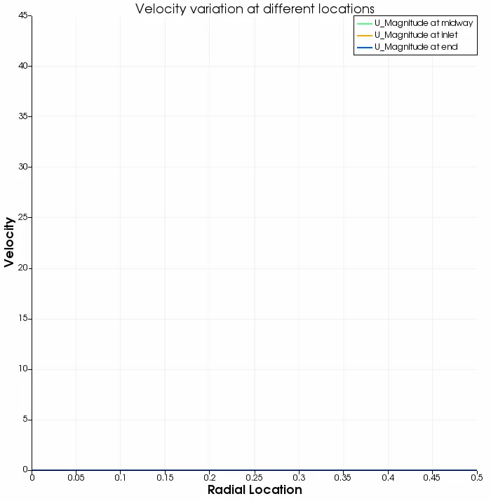
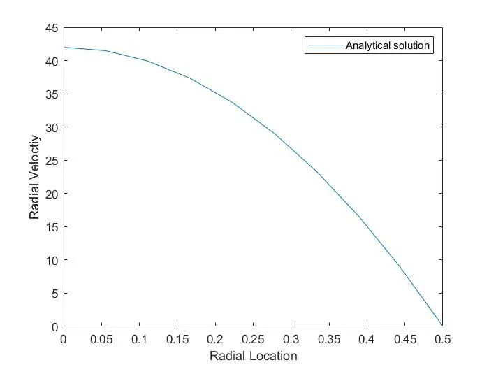
The straight vertical line at location 0.5m can be avoided by further refining the mesh.
Inlet (0.5m) - The velocity profile quickly stabilizes at the inlet. The velocity at the centre of the cylinder (0m or axis) is 21m/s, which is also the inlet condition provided by us. It quickly drops as we approach the walls and reaches zero i.e. No-slip condition.
Midway (100m) - The velocity profile stabilizes after some time at midway and reaches close to 41m/s at the axis. This is an indication that the flow is not fully developed (for a fully developed flow, Vmax =Vaxis =2*inlet velocity=2*21=42m/s). This can be verified by finding the analytical Hydrodynamic length (120m).
Outlet(199.5m) - The maximum velocity reaches 41.99 m/s at the axis. This means that the flow has fully developed.
It can be seen that the fully developed velocity profile is parabolic in both cases, which means our converged solution is a good one.
3. Pressure Drop
OpenFoam Generated Matlab Generated
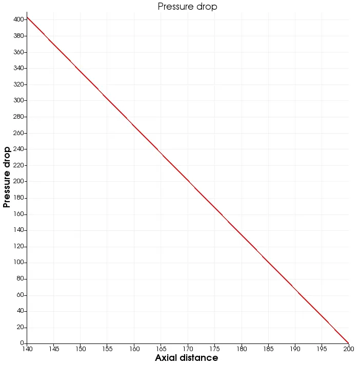
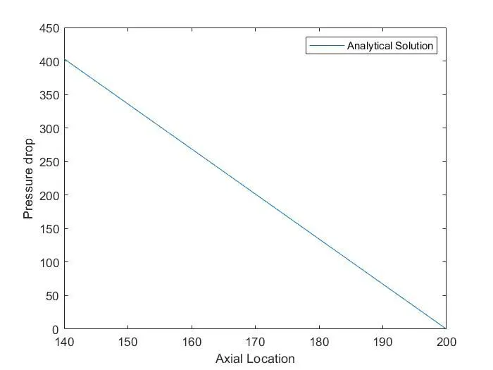
Here, the axial distance starts from 140m, because we are considering only the region where the flow is fully developed. The pressure drop at the end is zero, which is specified as an input property while solving this problem. The solution obtained using OpenFoam is consistent with the analytical solution, which was found using Matlab.
4. Shear stress
OpenFoam Generated
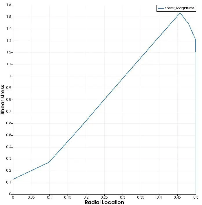
The shear stress plot obtained from OpenFoam makes sense because shear stress grows as we move from axial location to circumference. The Maximum shear stress from the plot is around 1.6, which goes hand in hand with the results obtained analytically using Matlab.
As promised at the end of case 3, the following is the blockMeshDict file for the Mesh shown in case 3
/*--------------------------------*- C++ -*----------------------------------*
  =========                 |
  \      /  F ield         | OpenFOAM: The Open Source CFD Toolbox
   \    /   O peration     | Website:  https://openfoam.org
    \  /    A nd           | Version:  9
     \/     M anipulation  |
*---------------------------------------------------------------------------*/
FoamFile
{
    format      ascii;
    class       dictionary;
    object      blockMeshDict;
}
// * * * * * * * * * * * * * * * * * * * * * * * * * * * * * * * * * * * * * //

convertToMeters 1;

r 0.9;
nr #calc "-$r";
l 40;
theta 45;
ct #calc "cos(degToRad($theta))";
st #calc "sin(degToRad($theta))";
a #calc "$r*0.33";	//half of side of square
na #calc "-$a";
rct #calc "$r*$ct";
nrct #calc "-$r*$ct";
rst #calc "$r*$st";
nrst #calc "-$r*$st";
ncur #calc "$na+(0.5*$na)";
cur #calc "$a+(0.5*$a)";
vertices
(
    (0 0 0)			//0 centre of inlet

    (0 $rct $rst) 		//1 cylinder inlet
    (0 $nrct $rst) 	//2
    (0 $nrct $nrst) 	//3
    (0 $rct $nrst) 	//4

    ($l 0 0) 			//5 centre of outlet

    ($l $rct $rst) 	//6 cylinder outlet
    ($l $nrct $rst) 	//7
    ($l $nrct $nrst) 	//8
    ($l $rct $nrst) 	//9

    (0 $a $a)			//10 inlet square (mesh)
    (0 $na $a)			//11
    (0 $na $na)		//12
    (0 $a $na)			//13

    ($l $a $a)			//14 outlet square (mesh)
    ($l $na $a)		//15
    ($l $na $na)		//16
    ($l $a $na)		//17
);

blocks
(
    hex (12 16 17 13 11 15 14 10) (20 10 10) simpleGrading (1 1 1)	//Square
    hex (11 15 14 10 2 7 6 1 ) (20 10 10) simpleGrading (1 1 1)	// East arc
    hex (13 17 9 4 10 14 6 1 ) (20 10 10) simpleGrading (1 1 1)	// North arc
    hex (3 8 9 4 12 16 17 13 ) (20 10 10) simpleGrading (1 1 1)	// West arc
    hex (3 8 16 12 2 7 15 11 ) (20 10 10) simpleGrading (1 1 1)
);

edges
(
 arc 1 2 (0 0 $r)	//inlet
 arc 2 3 (0 $nr 0)
 arc 3 4 (0 0 $nr)
 arc 4 1 (0 $r 0)

 arc 6 7 ($l 0 $r)	//outlet
 arc 7 8 ($l $nr 0)
 arc 8 9 ($l 0 $nr)
 arc 9 6 ($l $r 0)

 arc 12 13 (0 0 $ncur)
 arc 16 17 ($l 0 $ncur)

 arc 12 11 (0 $ncur 0)
 arc 16 15 ($l $ncur 0)

 arc 11 10 (0 0  $cur)
 arc 15 14 ($l 0 $cur)

 arc 10 13 (0 $cur 0)
 arc 14 17 ($l $cur 0)

);


boundary
(
    inlet
    {
        type patch;
        faces
        (
            (11 10 13 12)
            (11 2 1 10)
            (10 1 4 13)
            (13 4 3 12)
            (12 3 2 11)
        );
    }
    outlet
    {
    	type patch;
    	faces
    	(
    	    (15 14 17 16)
    	    (15 7 6 14)
    	    (14 6 9 17)
    	    (17 9 8 16)
    	    (16 8 7 15)
    	);
    }
    fixedWalls
    {
        type wall;
        faces
        (
            (2 1 6 7)
            (1 4 9 6)
            (4 3 8 9)
            (3 2 7 8)
        );
    }

);


// ************************************************************************* //
Conclusion
It can be concluded that the solution obtained from OpenFoam matches the analytical solution, obtained from Matlab.
References
- https://en.wikipedia.org/wiki/Hagen%E2%80%93Poiseuille_equation#Derivation
- https://www.youtube.com/channel/UCXAS_Ekkq0iFJ9dSUIkcAkw
- For understanding Viscosity - https://youtu.be/VvDJyhYSJv8
- https://www.openfoam.com/documentation/user-guide/a-reference/a.1-standard-solvers
- Matlab Documentation