Mixing Tee

AIM

To perform and analyze study state simulations of Tee joints in pipes, for various cases of pipe lengths and Momentum ratios and verify the results with Analytical values.

Hot inlet velocity = 3m/s
Hot inlet Temperature = 36 degrees
Cold inlet Temperature = 19 degrees

Case 1: Shorter Tee

1.1- Momentum Ratio = 2

1.2- Momentum Ratio = 4

Case 2: Longer Tee

2.1- Momentum Ratio = 2

2.2- Momentum Ratio = 4

Introduction

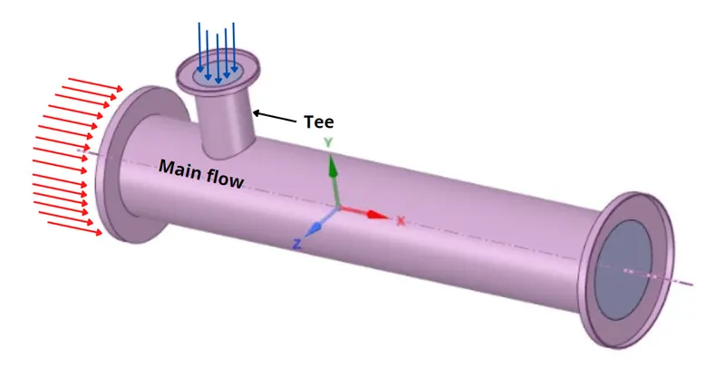
A mixing Tee is formed by joining two pipe sections at right angles to each other, to form a T-shaped geometry. This is a simple and cost-effective method to diffuse/mix two fluids. One fluid stream passes straight through the longer or main section, whereas the other fluid stream enters perpendicularly into the mainstream, causing a turbulent mixing action.

Applications

• Dilution of concentrated acids and bases.
• Injection of additives in fluids (usually petrochemical fluids).
• Wastewater treatment.
• Mixing of fluids at different temperatures to provide ambient temperature fluid. E.g. Air conditioners, Geysers. More sophisticated and efficient mixing methods have replaced the mixing Tee method for this particular use.

Characteristics

1. Velocity/Momentum Ratio

The momentum ratio is the ratio of velocity at the cold inlet to the velocity at the hot inlet.

It has been found that satisfactory mixing was obtained when the ratio of the velocity of side-to-main flow was in the range of 2 to 3.

2. Tee positioning

The mixing criteria in many of the experiments assumed that optimum mixing in a pipeline was achieved if the side jet was centered along the pipeline axis after entering the main flow.

3. Tee Angle

It was also found that good mixing characteristics can be achieved by varying the Tee angle. Tee angle also determines the minimum length of the pipe downstream of the Tee required for a good distribution/mixing.

4. Chemical composition

Chemical composition and nature of the fluids are important criteria, as they define if the fluids are reactive or non-reactive when mixed. For a reactive mixture, convection plays a significant role in the distribution of particles.

5. Material properties of the Tee

In heat transfer studies, the material properties of the Tee should also be taken into consideration, as a significant amount of heat transfer can take place through conduction.

Thermal stripping

When the temperatures of fluids entering the Tee are at huge temperature differences, large fluctuations in metal temperature can be observed, this can cause thermal fatigue of the Tee structure. This phenomenon is called Thermal stripping. Thermal stripping can also occur under steady-state conditions. If not properly designed, cracks can develop and can lead to fluid leaks.

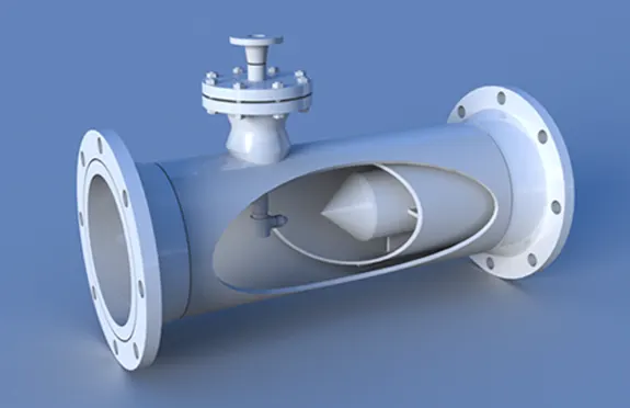
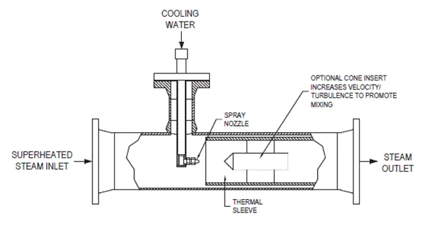
To avoid the problem of Thermal stripping, a thermal sleeve is placed near the walls where potential variation in temperature can arise.

Procedure

Pre-processing

1. Open Ansys Fluent and import the required Geometry.
2. Open Geometry and suppress the physics of parts, which do not impact the flow.
   Dimensions:
   Cold inlet diameter (Tee)=16.9626mm
   Hot inlet diameter (Main)=34.8761mm
3. Generate the Mesh and check for the Element quality of the Mesh. A good Mesh element has a quality of more than 0.05 or 5%.
   
   Default Mesh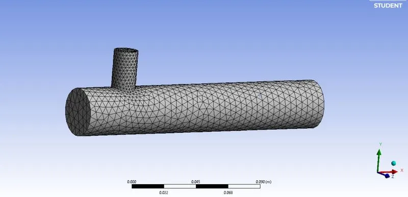
   
   
   
   
   Mesh Quality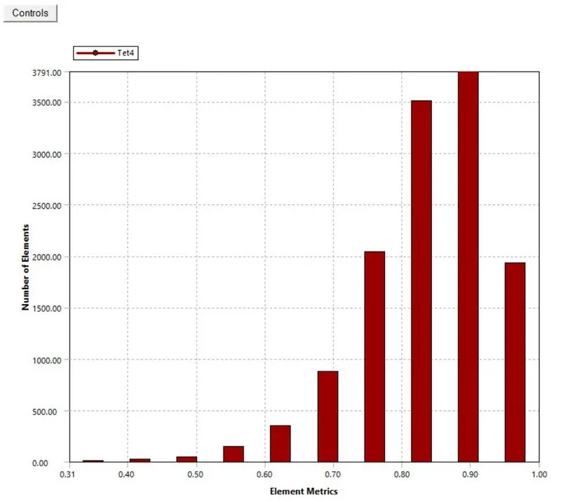
   
   
   
   The least quality element's element metrics value was higher than the 0.05 value, this explains that the mesh quality is good.
4. General options - Steady-state; pressure-based calculation.
   There is a pressure-based solver and there is a density-based solver. The choice depends on the velocity of flow we are dealing with.
   Density-based solvers calculate their timestep on the acoustic time scale. Since for low-speed flows, the relative speed of sound is very high. The time steps are required to be very small and thus increasing computational power and costs.
   Pressure-based solvers, on the other hand, calculate the time step based on the flow velocity and hence are cheaper for Low-Mach flows or incompressible flows.
   As we approach transonic speeds, the flow speed becomes comparable with the speed of sound, and pressure-based solvers become as expensive as density-based solvers. In addition to this, they tend to give out wrong results. So, Density-based solvers are a better option when it comes to high-speed flows or compressible flows.
5. Specify the names of the boundaries, boundary names must make logical sense, as Ansys predefines the boundary conditions as per the boundary names. Though the boundary conditions can be changed manually at a later point in time, it is a good practice to give names that make sense.

Processing

1. Open setup, select if the Energy equation needs to be solved (in this case -Yes), change the flow properties if required, or the default option is Air.
2. Specify the boundary conditions.
   Outlet pressure (gauge pressure) = 0 ; hot inlet velocity = 3m/s ; cold inlet velocity = based on the momentum ratio
3. Select the solver model, since we are interested in solving turbulence we use Standard K-Epsilon[9][10] and SST-K-Omega[11] models.
   Note-SST-K-Omega model uses K-epsilon solver away from the boundaries and K-Omega model near the boundaries.
4. Select the desired reports that are needed to be generated, In this case, they are, Weighted average and standard deviation of Temperature at the exit of the pipe.
5. Hybrid initialisation t=0;
   In standard initialization, the user has to guess the initial values, whereas, In hybrid initialization, the solver uses boundary conditions and Euler's equations and finds the suitable initial values.
6. Run the desired number of iterations.

Post-processing

Ansys provides tons of post-processing features, the ones used here are Temperature and Velocity based features.

Solver Selection and Grid Independence study

Which Turbulence Model is suited better? Standard-K-Epsilon or SST-K-Omega

Hot inlet Temperature = 36 degrees
Cold inlet Temperature = 19 degrees
Hot inlet velocity = 3 m/s
Momentum ratio = 2
Cold inlet velocity = Momentum ratio*Hot inlet velocity = 6 m/s
Number of nodes = 2825

Residuals

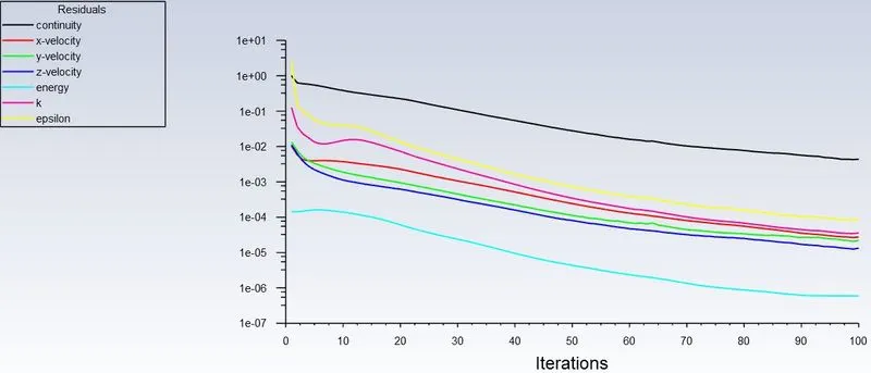
1. Standard-K-Epsilon
   
   
   
   
   
2. SST-K-Omega
   
   

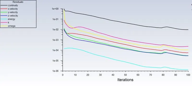
Lower Residuals = Good convergence.
The Residuals in the case of the standard K-Epsilon solver are smaller than the SST-K-Omega solver. So, standard K-Epsilon is better in this regard.
Also, it can be seen that convergence is achieved faster i.e. residuals drop faster, in the case of the Standard K-Epsilon model

Standard Deviation

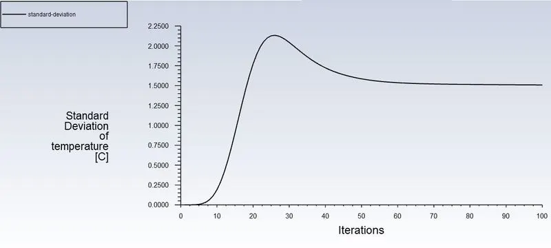
1. Standard-K-Epsilon
   
   
   
   
   
2. SST-K-Omega
   
   

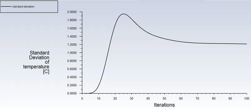
Standard deviation is a measure of the quality of mixing of the fluids. A lower standard deviation would mean better mixing.
So, if mixing is the criteria, then SST-K-Omega is a better option.

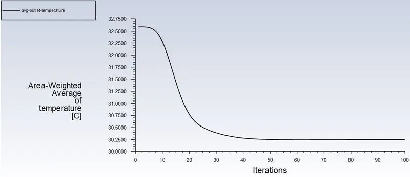
Average Temperature at the outlet

1. Standard-K-Epsilon
   
   
   
   
   
2. SST-K-Omega
   
   
   
   

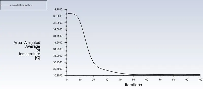
The final average steady-state temperature at the exit is the same no matter which solver is being used.

From the above plots and discussion, the model to be used depends upon the requirement. If computational cost is to be kept lower, then the Standard-K Epsilon model must be preferred. But, if better mixing of fluids is preferred, then the SST-K-Omega model can be used.
Since the final average temperature is the same in both cases, hereafter the Standard K-Epsilon model will be used throughout the project.

Grid independence study

Grid independence is achieved when the solution no longer changes or changes < 2% when the grid is further refined.
The variation of the solution of the above case for the number of nodes=2825,3135,8336

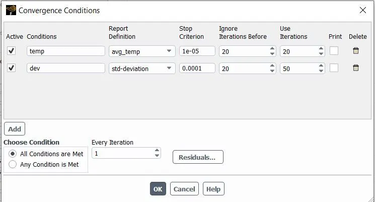
• Convergence Criteria

Usually, observing the residual plots and the parameter plots can help us tell when a solution has converged. But, this is prone to human errors. So, Ansys allows users to set the convergence criteria. The following conditions were set for this problem

Element size	Number of nodes	Number of elements	The iteration at which convergence is achieved	Average Temperature at the outlet
0.01 (default)	2825	12692	70	303.33986 k
0.005	3135	14249	110	303.393k
0.003	8336	39792	90	303.4162k

It can be observed that even when the number of nodes/elements is increased, there is not much change in the final steady-state temperature at the outlet. This means that grid independence has been achieved.

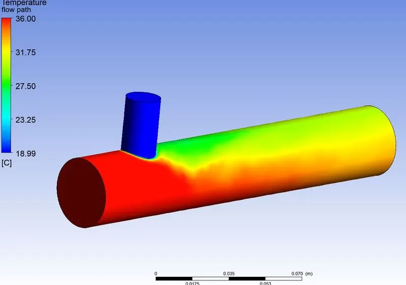
Simulation of Temperature distribution variation across each plane along the axis of the main pipe

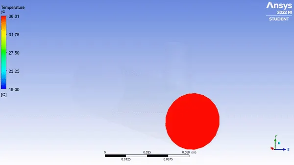
Temperature distribution of the flow in the pipe

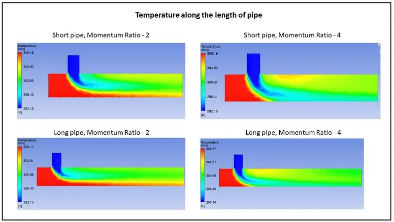
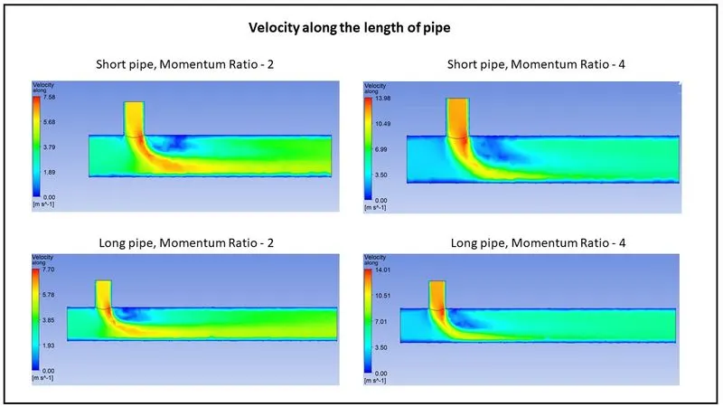
Results for different Momentum ratios and pipe lengths

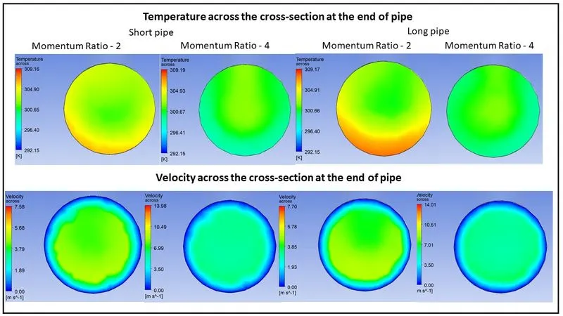
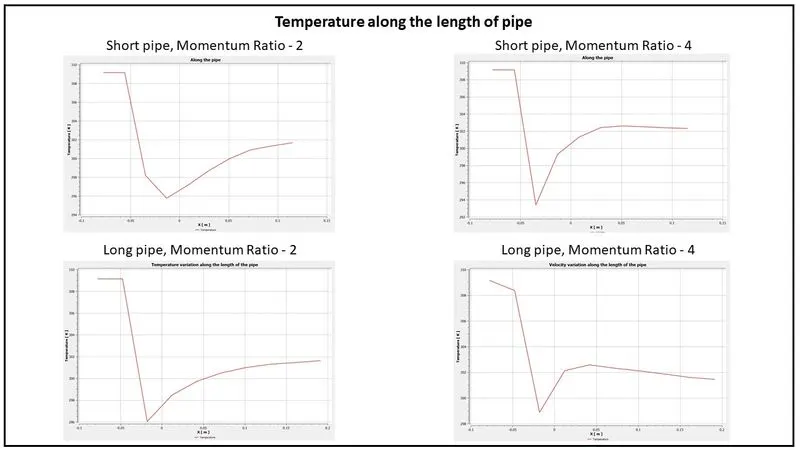
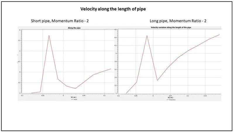
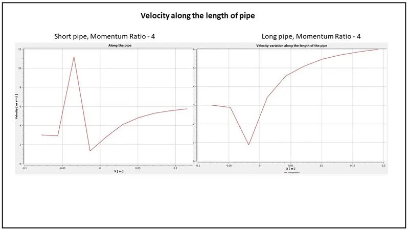
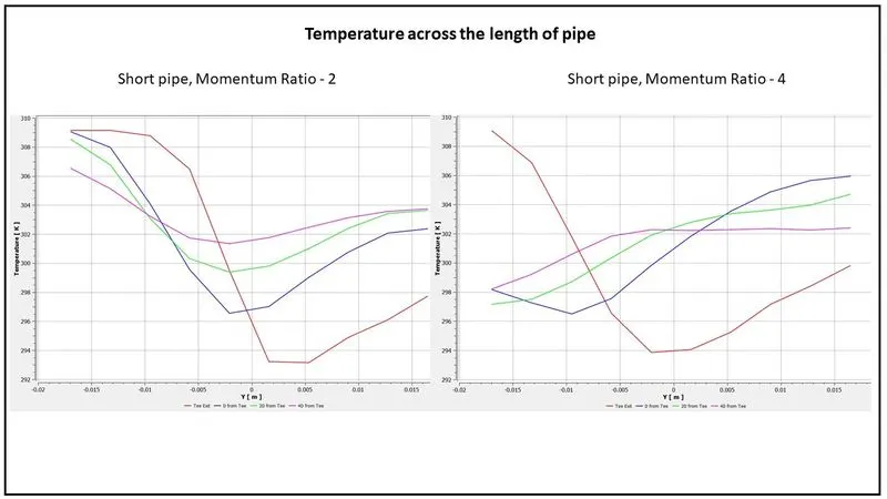
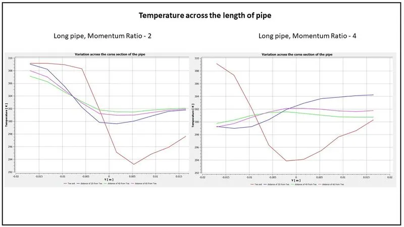
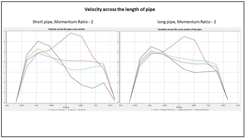
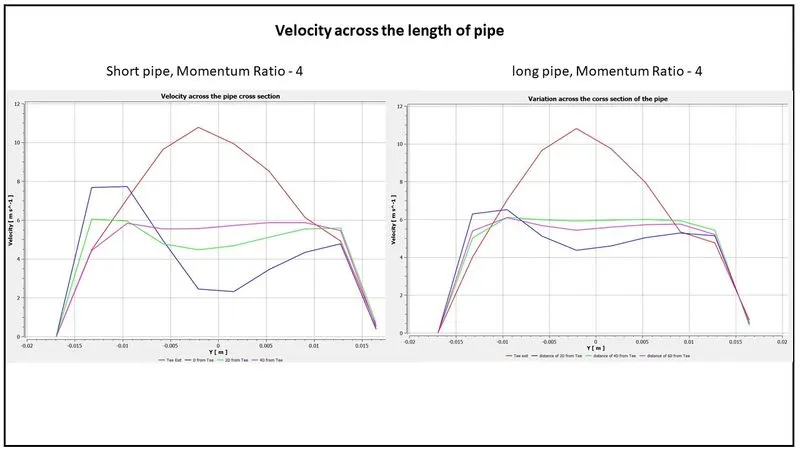
Pipe type	Momentum Ratio	Nodes	Cells/ Elements	Iterations	Temperature
Short	2	2825	12692	70	303.3398 K
Short	4	2825	12692	70	300.7031 K
Long	2	3479	15635	100	303.3981 K
Long	4	3479	15635	76	300.6397 K

Analytical Solution

For Momentum Ratios 2 and 4, the Temperature of the mixture would be 303.54023 k and 300.5 k respectively.

Conclusion:

1. K-Epsilon converges faster and thus is also cheaper. But, both converge at some point and give similar results.
2. The temperature drop is more when the Momentum ratio is high. A possible cause is turbulent mixing.
3. The numerical/computational solutions go hand in hand with Analytical solutions.
4. For best results, Longer pipe lengths and higher Momentum ratios can be preferred.

References:

1. http://www.virginiaheattransfer.com/content/heat-transfer/pickdesuperheater
2. https://becht.com/becht-blog/entry/cfd-modeling-of-mixing-tees-design-of-a-thermal-sleeve/
3. https://www.hydrocarbonprocessing.com/magazine/2020/august-2020/special-focus-valves-pumps-and-turbomachinery/cfd-modeling-of-mixing-tees-design-of-a-thermal-sleeve
4. https://becht.com/becht-blog/entry/cfd-modeling-of-a-mixing-tee-part-1-model-validation/
5. https://www.sciencedirect.com/science/article/pii/S0029549309005676
6. https://knowledge.autodesk.com/support/cfd/learn-explore/caas/CloudHelp/cloudhelp/2014/ENU/SimCFD/files/GUID-0F5C4828-9F91-46B6-A16A-2578D72DCFCC-htm.html
7. https://www.afs.enea.it/project/neptunius/docs/fluent/html/ug/node1022.htm
8. https://www.cfd-online.com/Wiki/RNG_k-epsilon_model
9. https://www.cfd-online.com/Wiki/K-epsilon_models
10. https://www.cfd-online.com/Wiki/Standard_k-epsilon_model
11. https://www.cfd-online.com/Wiki/SST_k-omega_model