Simulation of a 1D Super-sonic nozzle flow using Macormack Method in MATLAB
This project is about simulating flow in a C-D Nozzle using McCormack method for solving the conservative and non-conservative form of governing equations. To understand what is a conservative method and a non-conservative method, I strongly suggest the reader go through the works of JD Anderson or Malalashekara.
Note - To avoid clustering of plots, the lines/codes related to plots have been commented out, and the user may uncomment them as per requirement. The lines related to saving the animations are also commented out.
Before calling the function, do delete the values of L and n from the codes.
Function for Conservative form :
% Before using this function please uncomment the required plots.


function [r,v,T]=Nozzle_conservative(L,n)
n=31;
L=3;                    % Lenght of nozzle
x=linspace(0,L,n);     % Node positioning
dx=x(2)-x(1);           % Grid spacing
g=1.4;                  % Gamma
c=0.5;                  % CFL number
y=linspace(-6,6,n);

for i=1:length(x)              % Initial conditions
    if x(i)<=0.5
        r(i)=1;
        T(i)=1;
    elseif x(i)>=1.5
        r(i)=0.634-0.3879*(x(i)-1.5);
        T(i)=0.833-0.3507*(x(i)-1.5);
    else
        r(i)=1-0.366*(x(i)-0.5);
        T(i)=1-0.167*(x(i)-0.5);
    end
    T(i)=1;
    r(i)=1;
    A(i)=1+(2.2*(x(i)-1.5)^2);
    u1(i)=r(i)*A(i);
    u2(i)=0.59;
    v(i)=0.59/u1(i);
    u3(i)=u1(i)*((T(i)/(g-1))+(0.5*g*v(i)*v(i)));
    f1(i)=u2(i);
    f2(i)=((u2(i)*u2(i))/u1(i))+((g-1)/g)*(u3(i)-((0.5*g*u2(i)*u2(i))/u1(i)));
    f3(i)=((g*u2(i)*u3(i))/u1(i))-(0.5*g*(g-1)*(u2(i)^3/u1(i)^2));
end
ct=1;
for t=1:300                % timestep's as per convenince
    for i=1:length(x)
        a(i)=(T(i))^0.5;
        dt(i)=(c*dx)/(a(i)+v(i));
    end
    dt=min(dt);
    for i=1:length(x)-1     % Predictor Step
        J2(i)=(r(i)*T(i)/g)*((A(i+1)-A(i))/dx);
        pdu1dt(i)=-((f1(i+1)-f1(i))/dx);
        pdu2dt(i)=J2(i)-((f2(i+1)-f2(i))/dx);
        pdu3dt(i)=-((f3(i+1)-f3(i))/dx);
        pu1(i)=u1(i)+pdu1dt(i)*dt;
        pu2(i)=u2(i)+pdu2dt(i)*dt;
        pu3(i)=u3(i)+pdu3dt(i)*dt;
        pf1(i)=pu2(i);
        pf2(i)=((pu2(i)*pu2(i))/pu1(i))+((g-1)/g)*(pu3(i)-((0.5*g*pu2(i)*pu2(i))/pu1(i)));
        pf3(i)=((g*pu2(i)*pu3(i))/pu1(i))-(0.5*g*(g-1)*(pu2(i)^3/pu1(i)^2));
    end
    r=u1./A;
    v=u2./u1;
    T=(g-1)*((u3./u1)-(0.5*g.*v.*v));
    M=v./a;
    for i=2:length(x)-1     % Corrector step
        pJ2(i)=(r(i)*T(i)/g)*((A(i)-A(i-1))/dx);
        cdu1dt(i)=-((pf1(i)-pf1(i-1))/dx);
        cdu2dt(i)=pJ2(i)-((pf2(i)-pf2(i-1))/dx);
        cdu3dt(i)=-((pf3(i)-pf3(i-1))/dx);
        adu1dt(i)=0.5*(pdu1dt(i)+cdu1dt(i));
        adu2dt(i)=0.5*(pdu2dt(i)+cdu2dt(i));
        adu3dt(i)=0.5*(pdu3dt(i)+cdu3dt(i));
        u1(i)=u1(i)+(adu1dt(i)*dt);
        u2(i)=u2(i)+(adu2dt(i)*dt);
        u3(i)=u3(i)+(adu3dt(i)*dt);
    end
    u2(1)=2*u2(2)-u2(3);
    v(1)=u2(1)/u1(1);
    u3(1)=u1(1)*((T(1)/(g-1))+(0.5*g*v(1)*v(1)));
    u1(end)=2*u1(end-1)-u1(end-2);  % Boundary condition
    u2(end)=2*u2(end-1)-u2(end-2);
    u3(end)=2*u3(end-1)-u3(end-2);

    r=u1./A;
    v=u2./u1;
    T=(g-1)*((u3./u1)-(0.5*g.*v.*v));
    m=r.*v.*A;
    Mac=v./a;

    for i=1:length(x)
        f1(i)=u2(i);
        f2(i)=((u2(i)*u2(i))/u1(i))+((g-1)/g)*(u3(i)-((0.5*g*u2(i)*u2(i))/u1(i)));
        f3(i)=((g*u2(i)*u3(i))/u1(i))-(0.5*g*(g-1)*(u2(i)^3/u1(i)^2));
    end
    for i=1:length(x)
        for j=1:length(y)
            Mach(i,j)=Mac(i);
        end
    end

    %         figure(1)                 % Mach visualization with time
    %         pcolor(x,y,Mach')
    %         hold on
    %         colorbar
    %         caxis([0 3.5])
    %         shading interp
    %         plot(x,A,'color','k','linewidth',2)
    %         plot(x,-A,'color','k','linewidth',2)
    %         axis([0 3 -5.9 5.9])
    %         fill(x,A,'white')
    %         fill(x,-A,'white')
    %         text(1.2,-5,['Timestep=',num2str(t)])
    %         h=text(1.5,-1.2,['Mt=',num2str(Mac(16))]);
    %         set(h,'Rotation',90);
    %         m=text(0.1,-1.2,['Mi=',num2str(Mac(1))]);
    %         set(m,'Rotation',90);
    %         n=text(2.9,-1.2,['Me=',num2str(Mac(31))]);
    %         set(n,'Rotation',90);
    %         title('Mach variation in Nozzle')
    %         pause(0.001)
    %

%         figure(2)                 % Timewise variation
%         plot(x,r)
%         hold on
%         plot(x,v)
%         plot(x,T)
%         plot(x,m)
%         axis([0 3 0 2])
%         text(0.2,1.8,['Timestep=',num2str(t)])
%         title('Conservative Form - Timewise Variation')
%         legend('Density','Velocity','Temperature','Mass flow rate')
%         hold off
%     Mov(ct)=getframe(gcf);
%     ct=ct+1;
%
    r_throat(t)=r(16);
    T_throat(t)=T(16);
    v_throat(t)=v(16);

end

% movie(Mov)
% videofile=VideoWriter('Nozzle_cons_timewise.avi'); % change the file name as required
% open(videofile)
% writeVideo(videofile,Mov)
% close(videofile)

% figure(3)                     % Parameter - Timestep
% plot(r_throat)
% hold on
% plot(v_throat)
% plot(T_throat)
% legend('Density','Velocity','Temperature')
%
% figure(4)                     % Steady state distribution
% plot(x,r)
% hold on
% plot(x,v)
% plot(x,T)
% title('Conservative Form - Steady state Variation')
% legend('Density','Velocity','Temperature')
end
Function for Non conservative form :
function [r,v,T]=Nozzle_nonconservative(L,n)
n=31;
L=3;                    % Lenght of nozzle
x=linspace(0,L,n);     % Node positioning
dx=x(2)-x(1);           % Grid spacing
g=1.4;                  % Gamma
c=0.5;                  % CFL number

for i=1:length(x)              % Initial conditions
    r(i)=1-0.3146*x(i);
    T(i)=1-0.2314*x(i);
    v(i)=(0.1+1.09*x(i))*T(i)^0.5;
    A(i)=1+2.2*(x(i)-1.5)^2;
end
ct=1;
for t=1:300

    for i=1:length(x)
        a(i)=(T(i))^0.5;
        dt(i)=(c*dx)/(a(i)+v(i));
    end
    dt=min(dt);

    for i=2:length(x)-1
        dvdx(i)=(v(i+1)-v(i))/dx;
        drdx(i)=(r(i+1)-r(i))/dx;
        dTdx(i)=(T(i+1)-T(i))/dx;
        dlogAdx(i)=(log(A(i+1))-log(A(i)))/dx;
        drdt(i)=-r(i)*dvdx(i)-(r(i)*v(i)*dlogAdx(i))-(v(i)*drdx(i));
        dvdt(i)=-v(i)*dvdx(i)-(1/(g))*(dTdx(i)+((T(i)/r(i))*drdx(i)));
        dTdt(i)=-v(i)*dTdx(i)-((g-1)*(T(i))*((dvdx(i))+(v(i)*dlogAdx(i))));

    end

    for i=1:length(x)-1
        pr(i)=r(i)+dt*drdt(i);
        pv(i)=v(i)+dt*dvdt(i);
        pT(i)=T(i)+dt*dTdt(i);
    end

    for i=2:length(x)-1
        pdvdx(i)=(pv(i)-pv(i-1))/dx;
        pdrdx(i)=(pr(i)-pr(i-1))/dx;
        pdTdx(i)=((pT(i)-pT(i-1)))/dx;
        pdlogAdx(i)=(log(A(i))-log(A(i-1)))/dx;
        cdrdt(i)=-(pr(i)*pdvdx(i))-(pr(i)*pv(i)*pdlogAdx(i))-(pv(i)*pdrdx(i));
        cdvdt(i)=-pv(i)*pdvdx(i)-(1/(g))*(pdTdx(i)+((pT(i)/pr(i))*pdrdx(i)));
        cdTdt(i)=-(pv(i)*pdTdx(i))-((g-1)*(pT(i))*((pdvdx(i))+(pv(i)*pdlogAdx(i))));

        adrdt(i)=0.5*(drdt(i)+cdrdt(i));
        advdt(i)=0.5*(dvdt(i)+cdvdt(i));
        adTdt(i)=0.5*(dTdt(i)+cdTdt(i));

        r(i)=r(i)+(adrdt(i)*dt);
        v(i)=v(i)+(advdt(i)*dt);
        T(i)=T(i)+(adTdt(i)*dt);

    end

    v(1)=2*v(2)-v(3);
    v(31)=2*v(30)-v(29);
    r(31)=2*r(30)-r(29);
    T(31)=2*T(30)-T(29);

    m=r.*v.*A;
    r_throat(t)=r(16);
    T_throat(t)=T(16);
    v_throat(t)=v(16);
    m_throat(t)=m(16);

%     figure(5)                 % Time wise variation
%     plot(x,r)
%     hold on
%     plot(x,v)
%     plot(x,T)
%     plot(x,m)
%     axis([0 3 0 2])
%     text(0.2,1.8,['Timestep=',num2str(t)])
%     title('Non Conservative Form - Timewise Variation')
%     legend('Density','Velocity','Temperature','Mass flow rate')
%     hold off
%     Mov(ct)=getframe(gcf);
%     ct=ct+1;
%
end
% movie(Mov)
% videofile=VideoWriter('Nozzle_noncons_timewise.avi');
% open(videofile)
% writeVideo(videofile,Mov)
% close(videofile)

% figure(6)                     % Parameter - Nodal location (Steady state)
% plot(x,r)
% hold on
% plot(x,v)
% plot(x,T)
% legend('Density','Velocity','Temperature')
% title('Non Conservative Form - Steady state Variation')
% legend('Density','Velocity','Temperature')

end
Result
1. Steady-state
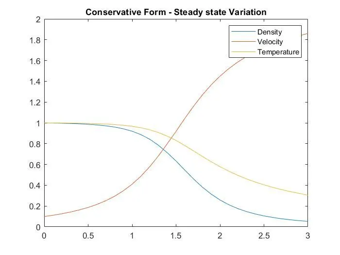
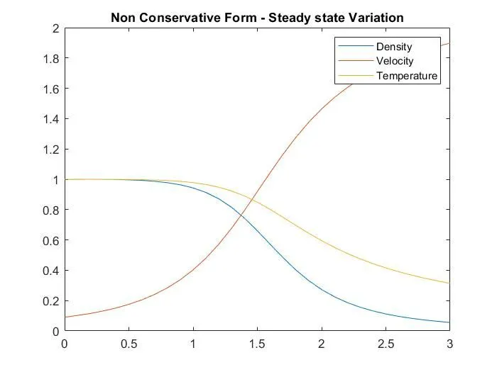
From the above graphs, it is clear that no matter what form of governing equations we use in this problem, the final steady solution is the same.
2. Timewise variation
Though the final steady-state solution was the same in both cases, the path in which the solution is obtained is completely different from each other. One of the forms might tend to converge faster than the other.
A.Conservative Form
B.Non conservative form
3. Nozzle flow simulation
It can be noticed from the simulation that, the Mach number at Throat does exceed 1 by a small margin. But this is not true in real-world situations. The mass flow at Throat chokes at Mach 1.
This is the reason why a C-D nozzle is chosen in the very first place for supersonic operations. A Convergent nozzle alone can never accelerate the flow over Mach 1, no matter how high is the pressure difference across it.