Week - 8 Mass Scaling

OBJECTIVE:

1. To see the impact of TSSFAC and DT2MS in *Control_Timestep card in a runtime for analysis.
2. Plot the Histogram to compare the runtime with mass scaling trials.
3. Study the behaviour with and without mass scaling with negligible deviation between results.
4. Compare the implicit and explicit run time for same simulation.

DESIGN OF EXPERIMENT:

Trial1: Running the model without *Control_Timestep. (Explicit)

Trial2: Running the model with *Control_Timestep. (Explicit)

Trial3: Running the model with different value of DT2MS. (Explicit)

Trial4: Running the model with different value of TSSFAC. (Explicit)

Trial5: Running the model for implicit analysis.

THEORY:

The timestep(t) for stress propogation in an element is defined as:

t = L/c

where,

L is length of element.

c is speed of stress propogation in element material.

c = `sqrt`(G/`rho`)

where,

G: Shear modulus

`rho`: density of material

G = E/2(1+v)

where,

E: Youngs Modulus for materal

v: poissons ratio

Timestep calculation by solver:

L is the length of smallest element in the model and hence using mass scaling, timestep can be increased for elements having greater L and simulation can be done at greater pace.

What if timestep is less than 't' ?:

't' is the minimum value of timestep which is feasible for an element with properties E,G,v and L.

If timestep is lesser than 't' then calculation for various parameters willnot be feasible and correct. Hence, to get the proper behaviour of model time step should be equal to more than 't'.

Smaller timestep will get finer results but will be computationally expensive, hence as a analyst it is very much important to get a value which computationally economical and optimum in magnitude to get better results (results which gives better behaviour results for model and is not computationally expensive and can be performed in optimum time.)

Mass scaling:

Mass scaling is a method by which analyst can increase the timestep by adding pseudo mass to an element. This results in faster simulation.

Disadvantages or precautions with Mass scaling:

Since added mass doesnot exist in reality hence there could be certain deviation from optimum results. So added mass is capped by magnitude for an analysis (Here it is capped at 8%)

Advantages with Mass scaling:

Total duration of simulation can be reduced significantly without any deviation from true behaviour of analysis.

Application of mass scaling:

Mass scaling is usually employed for explicit simulations as CFL equation is to determine min time step in explicit and in any case, an explicit simulation timestep should comply CFL.

Time step is very less for explicit but can be increased using mass scaling to get faster simulations.

TRIAL1: Solving model via explicit method without control timestep.

Keyword file is opened in Notepad++ and *Control_Timestep is put under comment using "$" symbol.

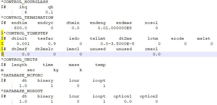
Command prompt window for the keyword file:

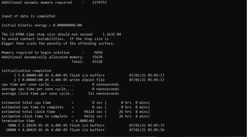
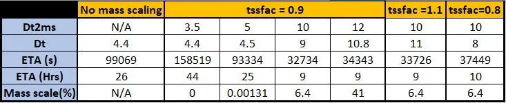
Estimated time to complete = 26 hrs 8 mins (99069 seconds)

Termination time = 6`times``10^2` seconds

Time step = 4.4`times``10^-5`seconds

TRIAL2: Solving model via explicit method with *Control_Timestep.

#1

tssfac = 0.9

dt2ms = -3.5`times``10^-5` seconds

so timestep = 3.5`times`0.9`times``10^-5` = 3.15`times``10^-5` seconds

So estimated finish time must increase because we have basically decreased the time step.

Command prompt window for the keyword file:

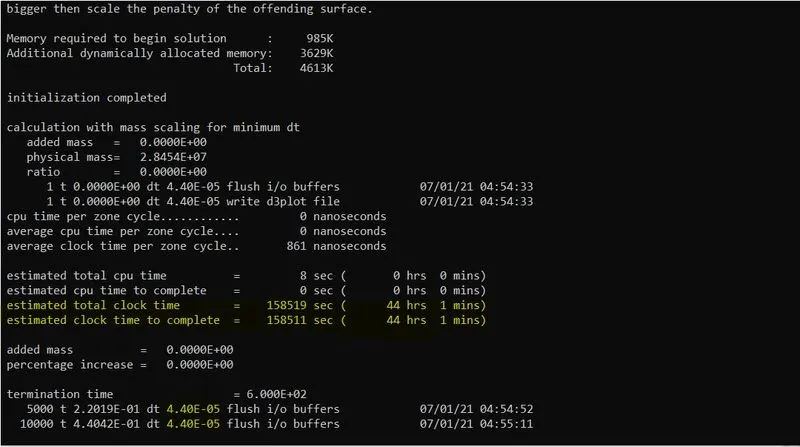
Estimated time to complete = 44 hrs 1 mins (158519 seconds)

Termination time = 6`times``10^2` seconds

Time step = 4.4`times``10^-5`seconds

There is no added mass since we have not increased timestep.

#2

tssfac = 0.9

dt2ms = -5.0`times``10^-5` seconds

so timestep = 5.0`times`0.9`times``10^-5` = 4.5`times``10^-5` seconds

So estimated finish time must decrease because we have slightly increased the time step.

Command prompt window for the keyword file:

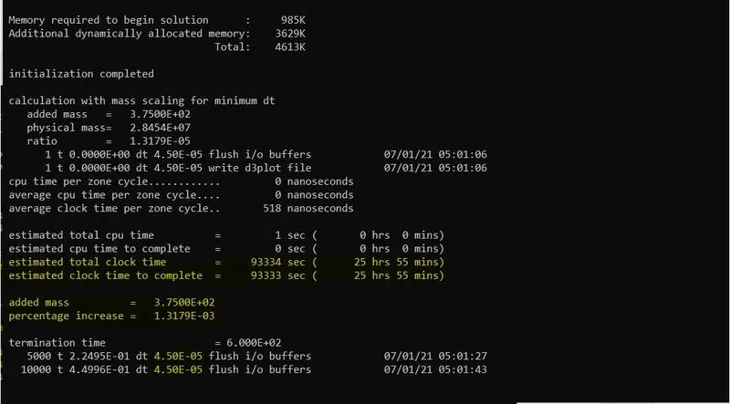
Estimated time to complete = 25 hrs 1 mins (93334 seconds)

Termination time = 6`times``10^2` seconds

Time step = 4.5`times``10^-5`seconds

Added mass in %age = 0.00131% which is highly negligible and hence we can certainly increase the time step.

Trial3: Running the model with different value of DT2MS.

#1

tssfac = 0.9

dt2ms = -1.0`times``10^-4` seconds

so timestep = 1.0`times`0.9`times``10^-4` = 0.9`times``10^-4` seconds

So estimated finish time must decrease because we have increased by an order of +10.

Command prompt window for the keyword file:

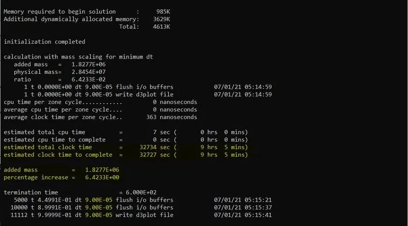
Estimated time to complete = 9 hrs 5 mins (32734 seconds)

Termination time = 6`times``10^2` seconds

Time step = 9.0`times``10^-5`seconds

Added mass in %age = 6.4% which is nearing our capped value of 8%.

#2

tssfac = 0.9

dt2ms = -1.2`times``10^-4` seconds

so timestep = 1.2`times`0.9`times``10^-4` = 1.08`times``10^-4` seconds

So estimated finish time must decrease because we have increased by 0.2

Command prompt window for the keyword file:

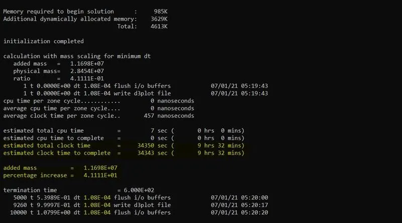
Estimated time to complete = 9 hrs 32 mins (34343 seconds)

Termination time = 6`times``10^2` seconds

Time step = 1.08`times``10^-4`seconds

Added mass in %age = 41.1% which is exceeding our capped value of 8% by a very high margin.

Trial4: Running the model with different value of TSSFAC.

#1

tssfac = 1.1

dt2ms = -1.0`times``10^-4` seconds

so timestep = 1.1`times`1.0`times``10^-4` = 1.1`times``10^-4` seconds

Command prompt window for the keyword file:

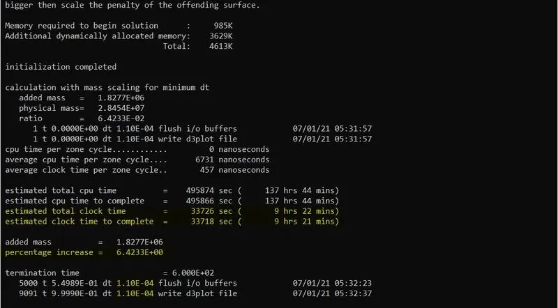
Estimated time to complete = 9 hrs 22 mins (33726 seconds)

Termination time = 6`times``10^2` seconds

Time step = 1.1`times``10^-4`seconds

Added mass in %age = 6.41% which is within our capped value of 8%.

By increasing tssfac we have increased timestep without increasing any mass%.

#2

tssfac = 0.8

dt2ms = -1.0`times``10^-4` seconds

so timestep = 0.8`times`1.0`times``10^-4` = 0.8`times``10^-4` seconds

Command prompt window for the keyword file:

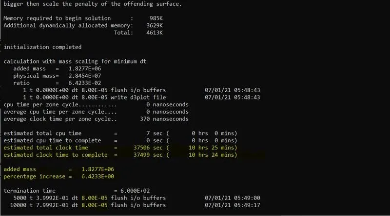
Estimated time to complete = 10 hrs 24 mins (37449 seconds)

Termination time = 6`times``10^2` seconds

Time step = 8.0`times``10^-5`seconds

Added mass in %age = 6.41% which is within our capped value of 8%.

By increasing tssfac we have increased timestep without increasing any mass%.

Trial5: Running the model using Implicit solving.

Problem solved in 2 seconds.

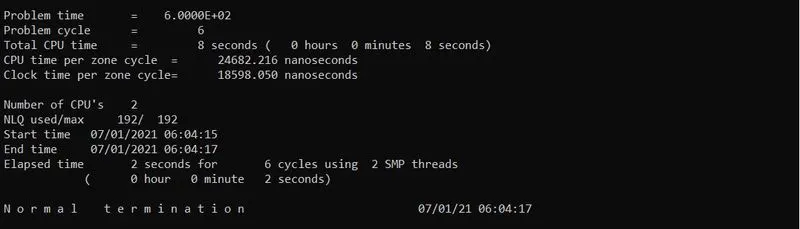
Implicit_General

imflag = 1 to avail implicit analysis

Implicit_Auto

iAuto =1

Dt = 0.001

Number of steps =1

Number of iterations =2

Histogram:

CONCLUSION:

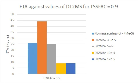
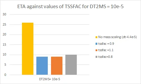
Using Mass scaling for Explicit analysis, we have successfully reduced the ETA from 26 hours to 9 hours.

Reduction in ETA (%age) = (26-9)/26 `times` 100 = 65.38 % in initial ETA.

Manipulating TSSFAC, DT2MS can be increased for explicit analysis, to reduce the solving time without any significant increase in added mass.

Keyword files are attached