Week - 8 Mass Scaling

Aim: To perform the Mass Scaling technique during solving the simulation by trial and error and then compare the results, also need to perform the same simulation with implicit approach.

Objectives:

Using the mass scaling technique to reduce the simulation time.

Perform the simulation with the Implicit approach

Note: Ensure mass scaling doesn’t cross 8% and the stability is intact, use best pair of DT2MS and TSSFAC to achieve this.

The time shown in this exercise is the preliminary estimated time shown by Ls-Dyna solver, also the actual time will be less than estimated time shown by the solver during solving the problem.

Theory:

Introduction to Mass Scaling in LS-Dyna [1]

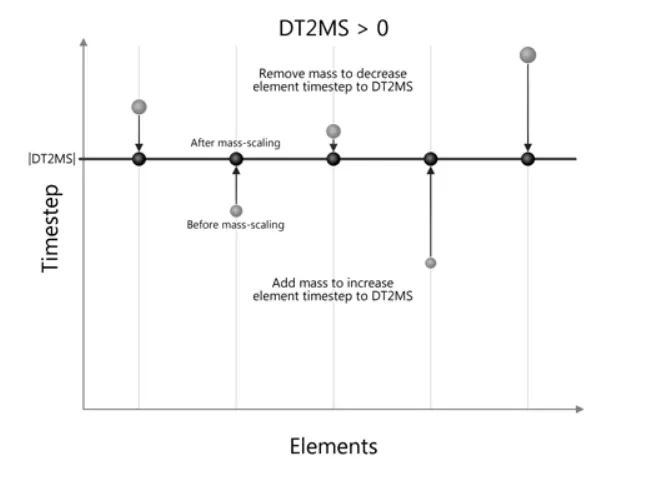
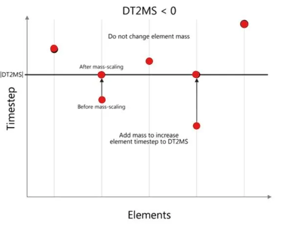
Mass scaling is a term that is used for the process of scaling the element’s mass in explicit simulation to adjust it’s time step. The primary motivation is to change (usually increase the global compute time step which is limited by the Courant’s stability criteria). LS-DYNA allows two different types of mass scaling using the DT2MS parameter from * CONTROL_TIMESTEP with the default set to no mass scaling, when DT2MS is less than 0, LS-DYNA add mass of each element whose time step is below DT2MS, such that element’s updated DT is equal to abs (DT2MS). When DT2MS is greater then zero, LS-DYNA add mass to those elements whose DT is below abs (DT2MS) and removes mass from those elements whose DT is above abs (DT2MS), DT2MS > 0 is not used regularly, where as the DT2MS < 0 is frequently used for overcoming the smallest computed timestep, care must be taken when using DT2MS < 0 to ensure that added mass doesn’t have an adverse effect on the simulation accuracy. It is common practice to limit the percentage of added mass to less than 5% (at parts level) in dynamics simulations. Optionally user can set ENDMASS in *CONTROL_TERMINATION to terminate a simulation based on percentage of added mass based on the total mass of the model, when END Mass is greater than zero, LS-DYNA terminates when percentage of added mass reaches END Mass and report of up to 20 nodes (Stored in descending order of its added mass due to mass scaling) is written to both standard output and D3HSP file. It should be noted that the percentage of the added mass is based on total mass of the model which included rigid wall and rigid body etc. LS-DYNA outputs the percentage of added mass at component level which is a better indicator of amount of added mass due to mass-scaling.

In other word we can say that mass scaling is refers to technique whereby nonphysical mass is added to a structure in order to achieve a large explicit timestep.

Anytime you add non-physical mass to increase the time step in a dynamic analysis, you affect the results, think of F = m*a, Sometimes the mass is insignificant, and in those case adding non-physical mass is justifiable. Examples of such cases may include the addition of mass to just few elements in a non-critical area or quasistatic simulations, where the velocity is low and kinetic energy is very small relative to the peak internal energy. In the end it is up to the judgement of the analyst to gage the affect of mass scaling, you may have to reduce or eliminate mass scaling in a second run to gage the sensitivity of the result to the amount of mass added.

One can employ mass scaling in a selective manner by artificially increasing material density of the part you want to mass scale. This manual form of mass scaling is done independently of the automatic mass scaling invoked with DT2MS in *CONTROL_TIMESTEP.

When DT2MS is input as a negative value mass is added to those elements whose timestep would otherwise less than DT2MS. By adding mass to these elements whose timestep become equal to DT2MS, An infinite number of combination of TSSFAC and DT2MS will give the same product, i.e. timestep but the added mass will be different of each of those combinations. The trend is that bigger DT2MS and smaller the TSSFAC, while TSSFAC*[DT2MS] = constant, the greater the added mass. In return, stability may improve as TSSFAC is reduced (Just as in non-mass scaled solution), the overall mass added is same but time to solve the problem increases because time step decreases as the factor is small. If stability is the problem with the default TSSFAC of 0.9, try 0.8 or 0.7, if you reduce TSSFAC, you can increase DT2MS proportionally so that their product, hence time step is unchanged.

To determine where and when mass is automatically added, write GLSTAT and MATSUM files. These files will allow you to plot added mass vs time for individual parts, respectively. To produce the fringe plot of added mass in parts comprised of shell elements (DT2MS negative), Set STSSZ = 3 in *DATABSE_EXTEND_BINARY. You can then fringe the added mass (per element) using LS-POST by choosing Fcomp > Misc > time step size (Here the label time step size is really the element added mass)

The concept of mass scaling for both option of DT2MS is graphically illustrated below.

Limiting Mass scaling to First Step:

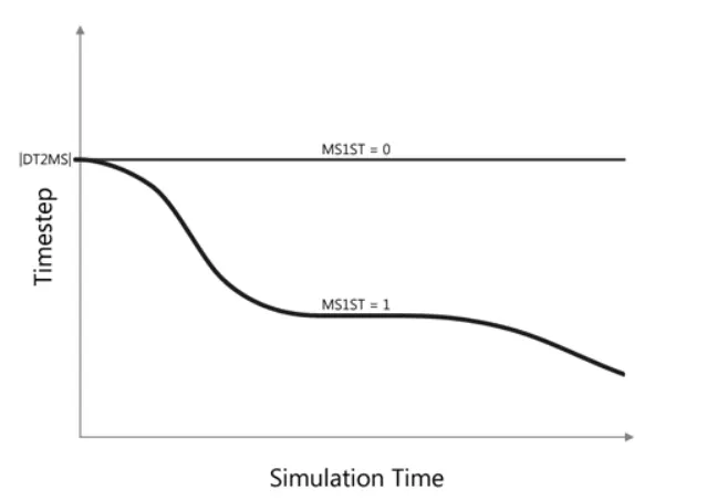
By default, when DT2MS is < 0, mass scaling is performed at every compute cycle (time step). When MS1ST (Mass-Scaling 1 Step) in *CONTROL_TIMESTEP set to 1, LS-DYNA will perform mass scaling only at first cycle. When this option is used, the time step will drop below abs (DT2MS), this is illustrated in the figure below

Dynamic Mass Scaling

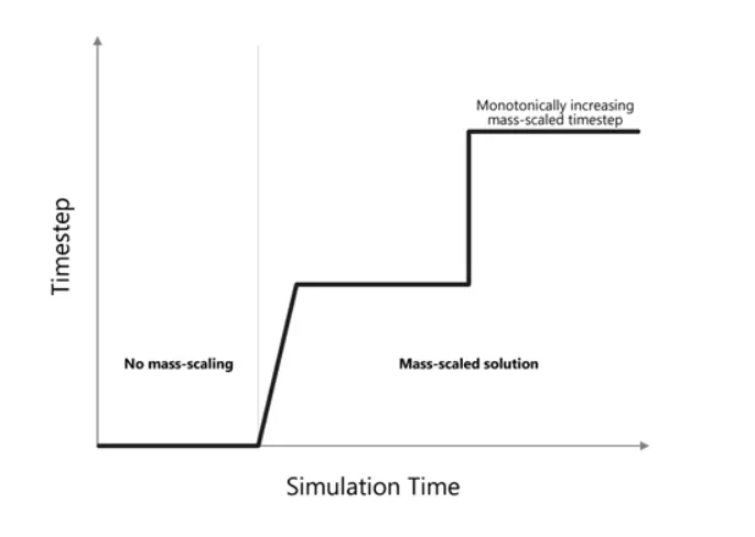
Mass scaling can also be specified by load curve with DT2MSLC parameter in *CONTROL_TIMESTEP. When DT2MSLC is greater than 0 it over rides the value of DT2MS, Load curve based mass scaling define using a monotonically increasing curve, is helpful when early part of simulation is dominated by inertia effects, and mass scaling during this time could affect the responses. In such case, a load curve based DT2MS can be defined with either a zero or small mass-scaled timestep can be input. It can be noted that ls-dyna always take the maximum of current time step and the ordinate value of the DT2MSLC to compute the mass scaling. A sample curve used by DT2MSLC as shown below.

Selective Mass Scaling:

Selective mass scaling which is much more accurate than default mass scaling, since it doesn’t scale the rigid body mass, selective mass-scaling can be turned on using the IMSCL in *CONTROL_TIMESTEP and could apply either to all the parts of the model (Set to 1) or do just a few parts (< 0 with abs (IMSCL) = part set list, which is recommended as the selective mass scaling is both, memory and CPU intensive.

Note: Amount of mass added to the element is governed by absolute value of DT2MS and is not multiplied by TSSFAC, For example, two different simulation with same DT2MS but with different TSSFAC will have the same percentage of added mass, then it is recommended to update DT2MS parameter directly and not TSSFAC (Time Step scale Factor)

Time Step Significance:

LS-Dyna calculates your solution by running over all the nodes in the model at each time step. In a very simplified explanation Ls-Dyna will look at the total force on each one from the previous time step, use that to find the acceleration of the of that node, and that to find the displacement of that node. The node is then moved by moved by this much. The calculation then updates the strain on the connecting element. This then goes through the material constitutive equation to get stress, which is applied as a force on the neighboring node in the next time step, we cam imaging this series of calculation behaving like wave, propagating through your mesh. The critical thing, however is you want to calculate all the node position of your model at the same time, without it being affected by the calculations from the previously calculated node. This basically means that you need to set your time increment such that code can calculate the displacement of the next node before the wave from the previous node calculation can hit it.

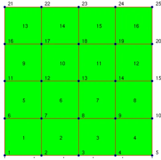
For instance if my boundary condition on the mesh below were along the left edges, an applied a downward load at node 25

the calculation at t = 0 as follow.

F at N25 = F0

This give acceleration (from F = ma with mass at 1/4^th the mass of element 16)

From acceleration we calculate the displacement for my next time step and move N25

Now the movement of this node imposes the strain on element 16 (from the material law) which will apply a force on N20, however we still not have calculated the displacement of N20 at t = 0, we have to do this before the wave propagating from N25 displacement hits N20

The wave travel through the material at the speed of the sound though that material, which depends directly on the density, Youngs Modulus and poison’s ration of that material.

The wave propagation velocity in a 2D shell element is given below

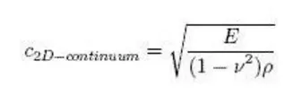
So the speed of sound through my material, and our mesh size determines how much time we have before to calculate displacement, Here we are using N20 as an example LS-Dyna also need to calculate N19 and N24 as the wave propagation in all directions.

So we have to take little margin of safety, means set my time step to exactly the time for wave to hit N20, it would be little risky and can lead to instability. Therefore LS-Dyna has a parameter in the *CONTROL_TIMESTEP card called as the TSSFAC, which is set to a default of 0.9, This is basically a scale factor on the calculated time step to ensure that N20 is calculate well in advanced of the wave front.

Now that makes sense for regular mesh. All the element have the same time step and every things work out great, what happen if our mesh is not regular, that what you see in most of time, because of the complexity of the geometry it is difficult to get the regular mesh having regular element size, we have some smaller elements, different material, affecting wave speed etc. This is unavoidable in real parts because of the necessity of capturing the geometry accurately. Then LS-Dyna will use the smallest time step calculated over all the element to ensure that none of the element get unstable, that means if we have one element with tiny step, the time step of your entire model is dictated by that one element increasing your computational cost and time to solve the problem.

This is why regular mesh and uniform mesh is better for when meshing an LS-Dyna model, and material with high wave propagation speed (generally metals) are meshed more coarsely than material with low propagation speed like plastic, rubbers, having finer mesh.

The list of 100 lowest time step is given in d3hsp file, search for smaller time step, and you should be able to find it in the file, use this list to see if you can re-mesh locally to remove small elements.

The other alternative is called mass scaling, here we artificially increase the mass of my smallest element and so increase the density of the element without affecting any other property, by this wave propagation speed is artificially reduced, increasing the time step for that element. So if we have a target time step for our entire model, LS-Dyna can look at which elements are below that time step and apply enough mass to those elements to ensure that their time step hits your target value. We can set the time step manually in the *CONTROL_TIMESTEP card under the DT2MS field.

Note: Mass scaling will allow you to setup the timestep, doesn’t mean that you can setup any value you want, remember we artificially increasing the mass in dynamic simulation as the analyses is progressing, it means that KE of that element is artificially going up, here LS-Dyna is creating energy from nothing. Ls-Dyna will output how much mass is added and shows the percentage of mass is added, for different problem this percentage of added mass will very from 5 to 8% but it is better to reduce this number as possible as much, because it greatly affect our results if our simulation is extremely fast and dynamic. The best way is to run the model without mass scaling and then run with mass scaling and compare the result to make sure the level of mass scaling and compare the results and time taken to solve the problem. This is the way in which Ls-Dyna calculate the time step, and also understand different method to increase time step or decreasing the solution time, on is using regular or proper mesh size and other is mass scaling technique to increase time step, The numerical stress wave must have always propagated less than one element width per time step, the above relation is called the Courant-Fedrichs-lewis (CFL) condition and determine the stable time step in an element. Basically CFL conditions express that the distance that any information travel during the time step length with in mesh must be lower than the distance between the mesh elements,

The CFL conditions requires that the explicit time step be smaller than the time needed by the physical wave to cross the element, 0.9 is the time step scale factor (TSSFAC), based on this the time step can be increase to provide the faster solution times by artificially increasing the density of the material by using technique like mass scaling, lowering the modulus or by increasing the element mesh.

Implicit vs Explicit Analysis [2]

Implicit and Explicit is differ in the approach to time incrementation, in implicit analysis each time incrementation has to converge, but we can set pretty long increments. Explicit on the other hand doesn’t have to converge each increment, but for the solution to be accurate time increment be supper small.

We can use Implicit and Explicit solver to sole the dynamic problems. Dynamic analysis will solve the problems involving inertial effects, those appear when thing change fast in our model like we are applying fast and quickly loads and impacts etc. generally called as Non-linear dynamics. Whereas linear dynamics problem are problem like Modal analysis or Forced response analysis that deals with vibrations.

We can start thinking about it not as a different solver but as a two different way of solving the same problem. In may cases we can use both implicit and explicit solve, and they will produce the same outcome.

How Dynamic Analysis Works?

Both of the analyses are solving a problem where the speed of things is important, this mostly means that load is applied fast, in such cases we will aways iterate our load in time, basically we will use the time to tell the solver what is happening and how the load is changing, firstly we have to define how the load is changing in time, we can define it by using curve like as shown below.

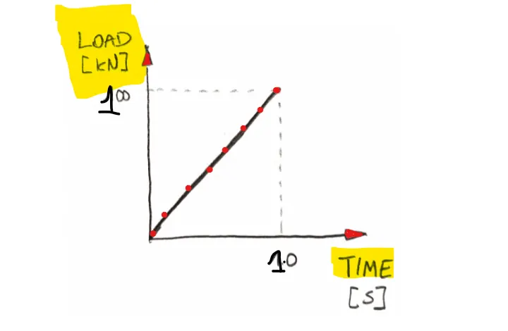
In non-linear dynamics time has two roles, first it allow us to tell the solver when how much load should be applied, we have to implemented each load with time dependent chart, Secondly time is time, It tells the solver how fast things are going.

Imagine we have such load sequence

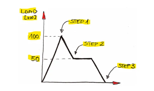
In static this would be 3 step analysis, the idea would be simple, we have to apply the 100KN of load in step 1 and then remove the 50 KN load in step 2 and then remove 50 KN load in step 3. There is no way to include the plateau of load after step 2 into the analysis, and it will be omitted, the logic is simple that no change in load = nothing changes in static.

Load increments in static

If the problem would be highly non-linear, the load would be incremented, it is rare to be able to apply full load into non-linear analysis at one go, this means that after 100 increments a full load of step 1 would be applied, this make easier for the solver to converge a correct answer, as a user we get to define how big increment solver should use. There are some algorithm to modify load incrementation during analysis, different solver have different way to do it. Usually FEA packages use load multiplier for this.

In Dynamic analysis we can get the load distribution as above with such load definition

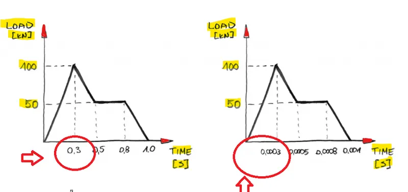
Here few things we need to notice

• There are no steps: This is because in dynamic analysis we won’t increment load, we will increment time, and since time goes constantly from zero to the prescribed value, we can increment it in one step
• Time is of the essence: When it comes to the value of the load, the above chart are the same, but it is not the same dynamic case, the chart on the right will apply a load 1000X quicker than left side, this isn’t something that we can ignore in dynamic analysis.

In general when we want to solve a dynamic problem, we are asking our solver to do one thing, we ask it to calculate the time increments, to see what is going on the model, in each of those increments time slightly increases, this off course also changes the load in the model, that’s why we need to have time dependent chart for the load, so the solver should know what load should be applied at which increment, to this extent it works the same as load increment in static analysis. The bonus is that we are incrementing time, inertia effect can taken into account, when things are happening fast enough.

To this extent, both implicit and explicit analysis does more or less same thing, they divide the analysis time into small increments, and then analyze what is going on the model, one increment of time after another, but here is where the similarities end, we see, there are different approaches to time incrementation we may have.

Implicit vs Explicit

We just leaned that in order to calculate the nonlinear dynamic problems, we will have to incrementally increase the analysis time, and there is two approaches to divide the analysis time into small increments first one is

Implicit Approach: Here in each time increment the global equilibrium in the model is established, this means that increment has to converge (this is happening in iterations)

After global equilibrium is established, solver calculates all the local finite element variables (Stresses etc.) for this increment.

Since Global equilibrium is verified at each time increment, those increment can be BIG

Drawbacks: Each time increment computes slowly, since iterations are needed to get the global equilibrium.

So if we are familiar with nonlinear static analysis, you will feel at home with the implicit solver, As a user, you usually get to say how big the time increments you want to have, this is huge advantage… that is easy to miss, because an explicit solver doesn’t offer such a possibility.

How Explicit Analysis work

It work in a way that we don’t have to converge each step, there are no convergence criteria, and no iterations, instead of verifying the global equilibrium solver assumes that the equilibrium simply exists. This mean that the solver goes straight into the calculation of local finite element variables, as such procedure has only one step.

• Calculate all of the local finite element variable for given increment and move to the next one.
• Benefits: Each increments calculates extremely fast
• Drawbacks: For this to work, the time step has to extremely small, otherwise it’s impossible to maintain this equilibrium that is assumed to simply exists. To achieve this, user don’t have direct control over how big-time increments explicit solver will take, Solver itself calculates how small time step are still ok, and those acceptable time increments are SUPPER SMALL, this is why explicit problems should last fraction of the second, if they would last seconds, you would need millions of increments.

So both implicit and Explicit solver solve the same stuff. The only difference is how those method increments time.

Technically both should produces the same outcome for all cases, after all we can analyze the same problem with both approaches. But it is not trivial thing, if the difference would be small, nobody would care to implement both, so let take a look at how the time incrementation influences things.

Both implicit and explicit solvers have some areas where they shine and there is an overlap in their use

• The implicit analysis allows you to select how big the time increment should be, this increment will take some time to compute since it has to iterate for global equilibrium first, but we can make it reasonably big for our analysis.
• Extreme time increments calculate really fast, simply because they don’t iterate for global equilibrium, but the time increment is not your choice, solver simply assumes that acceptable time increment is x and goes with it, this x can be something like 7 e -07 this is very small to solve the problem, an to solve a problem of 2s it would at least 4000000 increments.
• The speed of computing is exactly the difference between implicit and explicit, the size of explicit step will depend upon your model and computing time will depends upon hardware.

Use Implicit for Slow Analysis

If the things we calculate happens over several seconds, there is no sense in using explicit solver, it will take millions of time increments for this to compute, instead set reasonable time step for implicit analysis (let say 100 equal time increments for our analysis), sure each of those implicit time increment will compute much longer than single explicit increment, but not longer than hundred of thousand of them.

Use Explicit for Fast analysis

When calculated thing happens in fraction of second explicit is best, in an implicit analysis your time increment would be supper small, ma be as small as the increment in explicit analysis, in such a case explicit analysis will run much faster, since it doesn’t require global equilibrium iterations. The implicit analysis does require those iterations (regardless of time step). [2]

Procedure:

Mass scaling refer to technique where a non physical mass is added to the simulation in order to increase the timestep size and thereby decreasing the solution time. Since the run time is a function of density which in turn is a function of mass. Here we add artificial mass which might be affect our simulation results, so generally 5 to 8% of additional mass can be considered effective without much altering the solution as a whole in LS-Dyna, this can be done using CONTROL_TIMESTEP keyword by altering the value of DT2MS and TSSFAC values.

DT2MS: This parameter is used to define the new timestep of the simulation an thus affect the additional mass provided for the simulation.

Ideally the value of DT2MS < 0 to ensure that only negative value of dt are adjusted, where as positive value means those values which are above the time step should remain same as it is, this yield us a resultant positive mass.

TSSFAC: This parameter doesn’t effect the mass scaling, it basically used to relax the solver, it affects the timestep and thus simulation speed, it is the timestep factor that is multiplied with DT2MS to get the new time step

Time step dt = DT2MS*TSSFAC

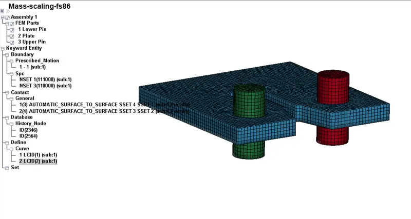
Defined problem

Explicit Approach:

1. Without mass scaling, i.e. DT2MS = 0

Here we can remove the control time step keyword or may be define we can define the value of DT2MS = 0 in Ls-Pre-post.

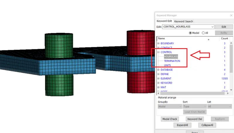
One easier way to change the value and temporary removal of Control time step card is commenting out in the file directly, that means commenting out the Control time step keyword, now by this our simulation become free from any mass scaling technique.

Commenting out the Control time step

Without mass scaling, i.e. DT2MS = 0

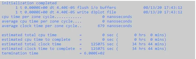
From the image we can see that estimated simulation time without mass scaling is 34hrs 44 min, so upon doing mass scaling we expect to gradually reduce the simulation time without adding more than 8% of the mass.

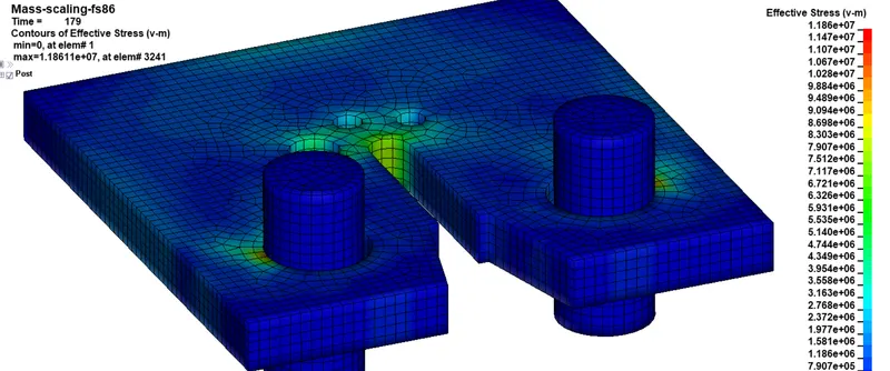
Ideally in order to verify the stability of the system, values of stress, strains, displacements should remain unchanged. Here stability criteria can be verified by ensuring that the timestep dt is not changed drastically, and this can be achieved by using TSSFAC card.

With Mass Scaling TSSFAC = 0.9 and varying DT2MS

DT2MS = -3.5e-05

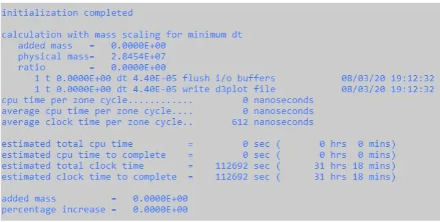
DT2MS = -5e-05

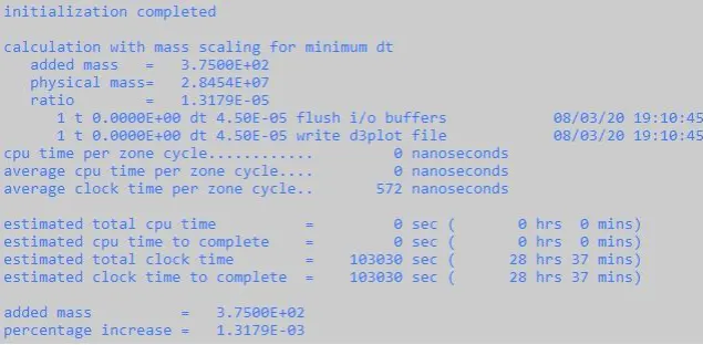
Percentage increase = 1.3179 E-03

DT2MS = -7e-05

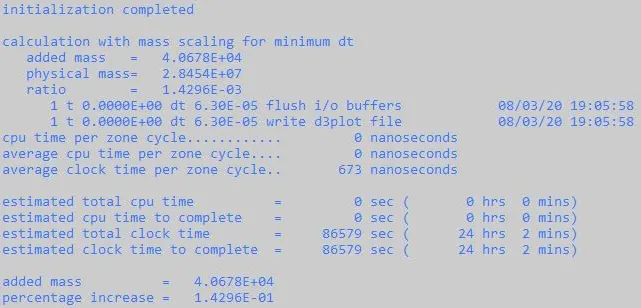
Percentage increase in mass = 1.42E-01

DTMS = -1.0e-04

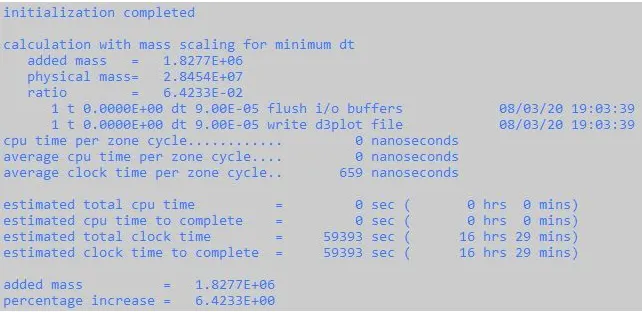
Percentage increase in mass = 1.827E+06

DT2MS = 1.03e-04

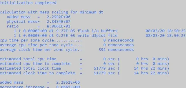
Percentage increase in mass = 8.061 E+00

DT2MS = 1.028e-04

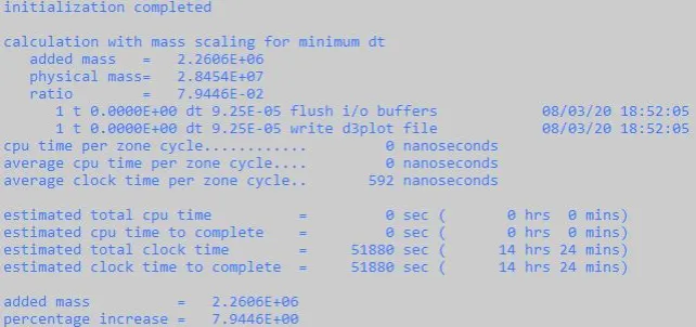
Percentage increase in mass 7.94 E+00 (Close to 8 value)

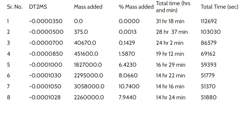
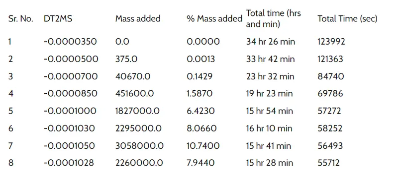
At DT2MS 1.03e-04 percentage increase in mass reaches to 8 value, that means mass is added up to 8% when we take time step value of 1.03e-04, it is better to not go beyond that limit.

Below table shows the result of different cases with TSSFAC of 0.9

With Mass Scaling TSSFAC = 0.8

DT2MS = -3.5e-05

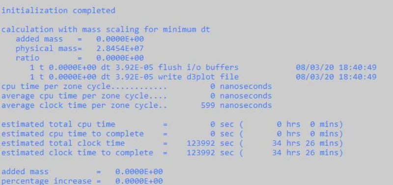
DT2MS = -5e-05

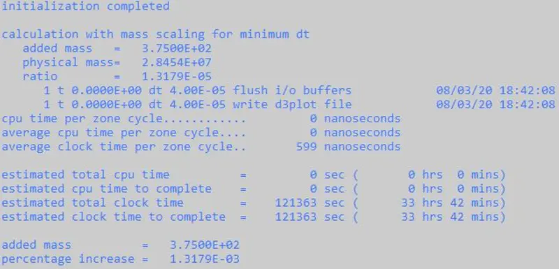
Percentage increase in mass = 1.31 E-03

DT2MS = -7e-05

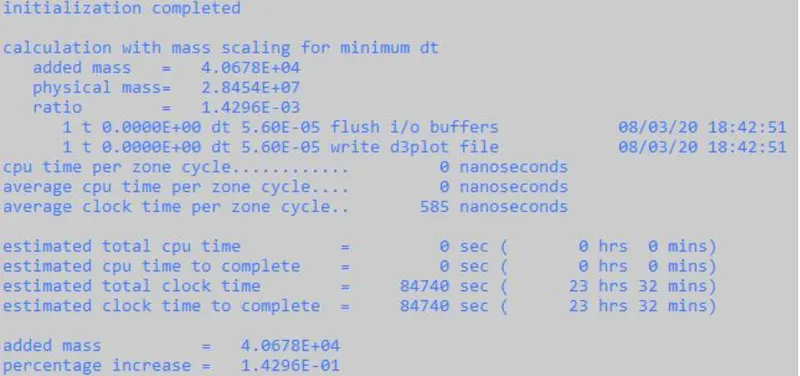
Percentage increase in mass = 1.42 E-01

DT2MS = -8.5e-05

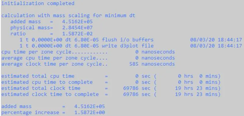
Percentage increase in the mass = 1.587 E+00

DT2MS = -1.0e-04

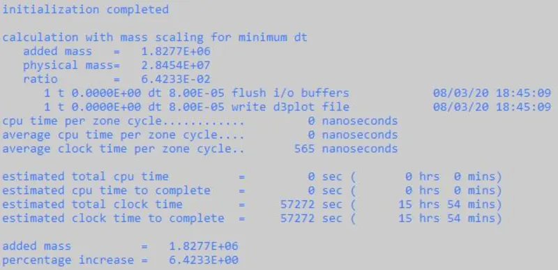
Percentage increase in the mass = 6.42 E+00

DT2MS = -1.03e-4

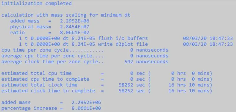
Percentage increase in mass = 8.06 E+00

Below table shows the result of different cases with TSSFAC of 0.8

Below graph shows the brief comparison for the DT2MS vs Running time for TSSFAC = 0.9 or 0.8

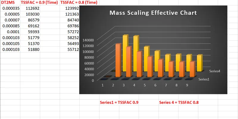
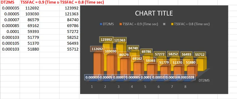
This will show that Mass scaling greatly affect our solution time and decrease the solution time, up to some extent, also large percentage of additional mass may leads to error as it leads to produce inertia effect in dynamic situation.

Implicit Approach

Now we will solve the same problem by using the implicit approach

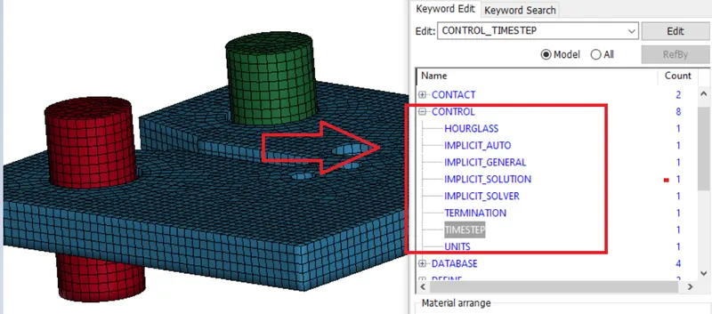
Defining the important Keyword for implicit analysis

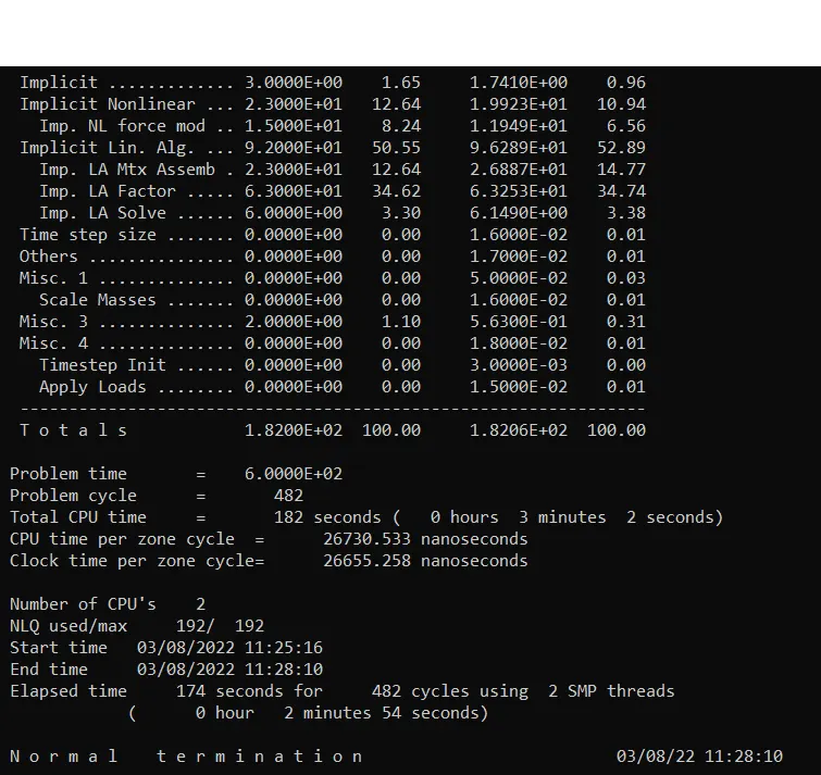
Here time to solve the problem decreases, because of having large time step value in case of implicit analysis, basic thumb rule to calculate the initial time step for implicit analysis is Termination time / 100, and we need to define this in Control implicit general which is essential keyword for starting the implicit analysis because ls-dyna is by default solve problem by using explicit approach, so we have to define the CONTROL_IMPLICIT_GENERAL Keyword to start the solution by implicit approach.

Conclusion:

• Using Mass Scaling techniques, we reduce the simulation time by adjusting the time step which is limited by courant’s stability criteria.
• Here we notice how DT2MS and TSSFAC will affect the simulation run time, DT2MS will basically affect the Mass Scaling, means percentage increase in mass depends upon DT2MS value, that is the time step value we defined, smaller the value more time required to solve the problem, because smaller the time step, and smaller the mass addition, by increasing the value, timestep value increases, and adding mass to those element whose time step is small, and decreasing the overall simulation run time, whereas the TSSFAC doesn't effect the mass addition, it basically reduce the timestep by some factor, so that problem shoud solve in a stable manner, It is observed that with same value of DT2MS, if we decreasing the value or TSSFAC, the mass addition would be remain same, but time to solve the problem would increases, because it gives relaxation for maintain stablity, the default value of TSSFAC is 0.9 and it can goes up to 0.6.
• In implicit analysis each time step has to converge, but we can set pretty long increment, on the other hand explicit doesn’t have to converge each time step, but for accurate solution time step must be very small, so time taken by Implicit approach to solve the above problem is less than explicit approach, also we can tweak the ITEOPT and ITEWIN option in CONTROL_IMPLICIT_AUTO to faster the solution time by using implicit approach.
• Use best pair of DT2MS and TSSFAC will gives us better result without affecting the stability and accuracy of the solution.

References:

[1] Ls-Dyna support

[2] https://enterfea.com/implicit-vs-explicit/