Week 7 State of charge estimation
AIM
- To stimulate 3 test cases from harness dashboard and study the results in detail.
- Understand about coulomb counting and study how BMS implements coulomb counting for SOC estimation
THEORY
SOC Estimitation methods
Extended Kalman Filter (EKF)
The Extended Kalman Filter (EKF) is a variant of the Kalman Filter that can be used to estimate the state of a dynamic system when the system dynamics and/or measurement models are nonlinear. The EKF is an approximation of the nonlinear system that uses the first-order Taylor series expansion to linearize the nonlinear functions around the current state estimate.
Like the standard Kalman Filter, the EKF is a recursive algorithm that estimates the state of a dynamic system based on measurements of that system. However, the EKF assumes that the system dynamics and measurement models are nonlinear, and it linearizes these models by approximating them with a linear model.
The EKF works by using the current state estimate and covariance matrix to linearize the nonlinear functions in the system dynamics and measurement models. Specifically, the EKF uses the Jacobian matrix, which is the matrix of partial derivatives of the nonlinear functions with respect to the state variables, to linearize these functions. The Jacobian matrix is evaluated at the current state estimate, which is used as the linearization point.
Once the nonlinear functions have been linearized, the EKF uses the Kalman Filter equations to update the state estimate and covariance matrix. These equations are modified to account for the nonlinearities in the system dynamics and measurement models.
One of the main advantages of the EKF is that it can be used to estimate the state of a nonlinear system using only the measurements from the system. This is particularly useful in cases where the system is too complex to be modeled analytically, or when the nonlinearities are too complex to be handled by other nonlinear estimation techniques.
However, the EKF has several limitations. First, the EKF is only an approximation of the true nonlinear system, and the accuracy of the estimates depends on the quality of the linearization. In some cases, the linearization may not be accurate, and the EKF may produce unreliable estimates. Second, the EKF can be computationally expensive, particularly for high-dimensional systems, as it requires the calculation of the Jacobian matrix.
Unscented Kalman Filter (UKF)
The Unscented Kalman Filter (UKF) is a variant of the Kalman Filter, which is a mathematical algorithm used for recursive estimation of the state of a dynamic system. The UKF is particularly useful when the system dynamics are nonlinear and the noise is non-Gaussian.
The UKF uses a set of sigma points to approximate the nonlinear functions and their associated covariance matrix in the system dynamics and measurement equations. These sigma points are chosen in a way that preserves the first and second moments of the distribution.
The UKF then propagates these sigma points through the nonlinear functions and calculates their mean and covariance. These are then used to update the predicted state estimate and the associated covariance matrix using the Kalman Filter equations.
The UKF has several advantages over other nonlinear estimation techniques. It is more accurate than the Extended Kalman Filter (EKF) in many cases, and it does not require the calculation of the Jacobian matrix, which can be computationally expensive. Additionally, the UKF can handle non-Gaussian noise models, which is a significant advantage in many real-world applications.
One of the key advantages of the UKF is that it does not require the calculation of the Jacobian matrix, which can be computationally expensive, particularly for high-dimensional systems. Instead, the UKF uses the sigma points to approximate the nonlinear functions, which can be much more computationally efficient.
Another advantage of the UKF is that it can handle non-Gaussian noise models. In many real-world applications, the noise may not be Gaussian, and the ability to handle non-Gaussian noise can be a significant advantage.
Coulomb counting
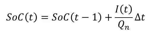
Coulomb counting is a technique used to estimate the amount of charge that has been delivered or removed from a battery by monitoring the flow of electrical current over time. In other words, it is a method of tracking the movement of electrons into or out of a battery, in order to determine the amount of charge that has been transferred.
The process involves measuring the current flowing into or out of the battery over a period of time, and then integrating the current measurement over that time period. This integration gives an estimate of the total charge that has flowed through the system.
Coulomb counting can be used to monitor the state of charge of a battery, and is often used in battery management systems to prevent overcharging or overdischarging of the battery. It is also used in electronic devices to estimate the remaining battery life, by measuring the amount of charge that has been used and comparing it to the total capacity of the battery.
Method of Coulomb counting by BMS
Battery Management Systems (BMS) use Coulomb counting to estimate the State of Charge (SOC) of a battery. The SOC is an important parameter that describes the amount of energy remaining in the battery, relative to its total capacity.
To implement Coulomb counting for SOC estimation, the BMS first measures the current flowing in and out of the battery over a certain period of time. This is typically done using a shunt resistor or a Hall-effect sensor to measure the current, and an Analog-to-Digital Converter (ADC) to convert the analog signal into a digital signal that can be processed by the BMS.
The BMS then integrates the current measurement over time, to estimate the amount of charge that has flowed into or out of the battery during that time period. This charge measurement is then used to update the SOC of the battery.
However, Coulomb counting is not a perfect method, as it can suffer from errors due to factors such as measurement inaccuracies, temperature variations, and changes in battery chemistry over time. To improve the accuracy of Coulomb counting, BMS may use additional methods such as temperature compensation and voltage-based estimations to refine the SOC calculation.
Modified Coulomb Counting Method
The modified Coulomb counting method uses the corrected current to improve the accuracy of estimation.
The corrected current is the function of discharging current. There is a quadratic relationship between the corrected current and discharging current of battery. By practice of experimental data, corrected current is calculated by the following form:

where k2,k1andk0">k2,k1andk0 are constant values obtained from the practice experimental data.
In modified Coulomb counting method, SOC is calculated by the following equation:
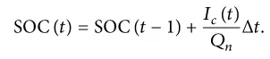
The experimental results show that the accuracy of the modified Coulomb counting method is superior to the conventional Coulomb counting method.
But there are several factors that affect the accuracy of Coulomb counting method including temperature, battery history, discharge current, and cycle life .
SIMULINK MODEL
Closed Loop Harness Dashboard
MODEL EXPLAINATION
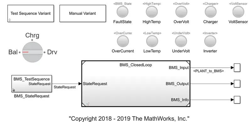
- The model shows battery model harness dash board.
- It consist of Test sequence variant block which is used to select any one of the three test case which is need to stimulate.
- The BMS state request blocks shows each sequences that is set in the stimulation at particular time in seconds.
- The model constist of fault state indicator, which shows in red whenever any fault in the system encounters otherwise it will be shown in green if no error encountered.
- The other indicators are high temperature,low temperature,under voltage,over voltage,voltage sensor,over current and inverter.Any of abnormality occours the each will be turned red and will remain green if everything is fine.
Initlizing
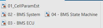
02-BMS System :
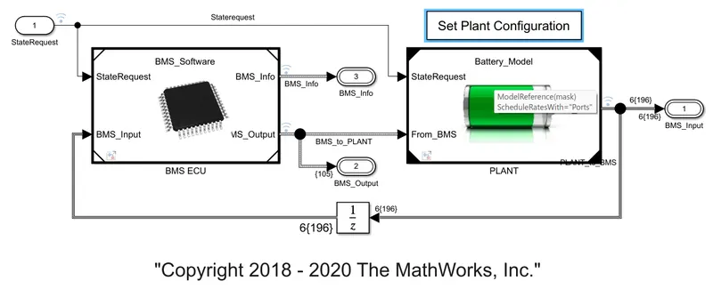
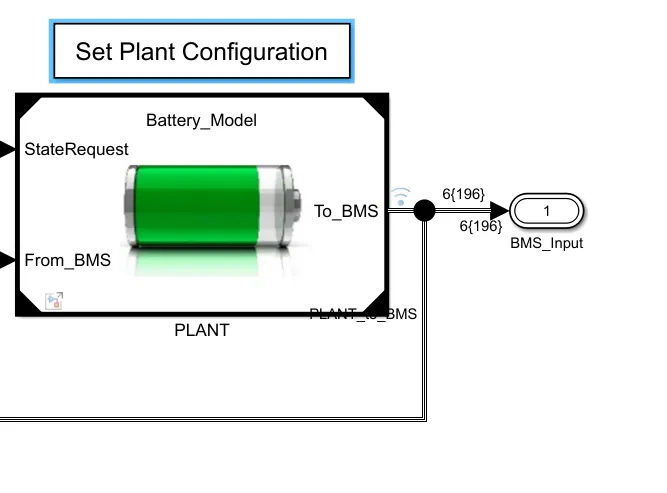
- First of all we need to select the battery pack required for the stimulation model.
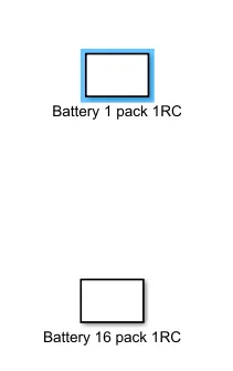
- There are two battery packs avaliable in the model, one is 1 battery pack which consist of 6 cells connected in series.
- The next configuration consist of battery with 16 packs, which consist of 16 battery packs connected in series each having 6 cells in series connection.
- For selecting the battery pack we need to go into 'Set Plant Configuraion' block where we can see two battery packs avaliable.
- To select the pack double click on the required pack.Here battery with 1 pack 1RC is selected for stimulation
Test case 1 Stimulation
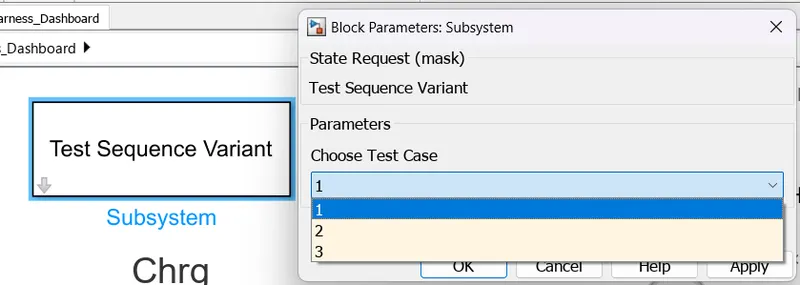
The test case 1 is selected by going to the Test sequence variant block and selecting 1 from the choose test case drop down list.
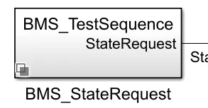
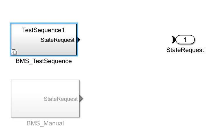
Now if we check the BMS state request block we can see the sequences and its timing of drivin,charging and standby conditions.
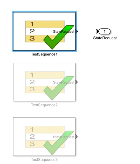
- Here we can see that the Test Sequence 1 has got highlited,it is because we have selected the 1 st test case from the test sequence variant block.
- This will change according to the test case selection automatically.
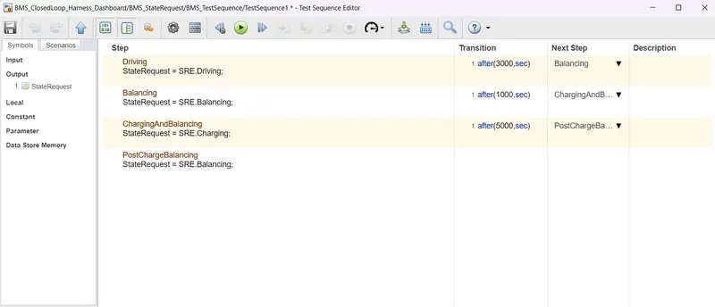
- When we get into the Test Sequence1 we can see that when the stimulation starts the vehicle will be in driving condition and after 3000 seconds the next step assigned is cell balansing mode or standby mode.
- It will last for 1000 seconds and after 1000 seconds the next step is changing and blancing mode.It will last for 5000 seconds.
- After 5000 seconds the next step is post balancing.
After simulating the model for 20000 seconds case 1
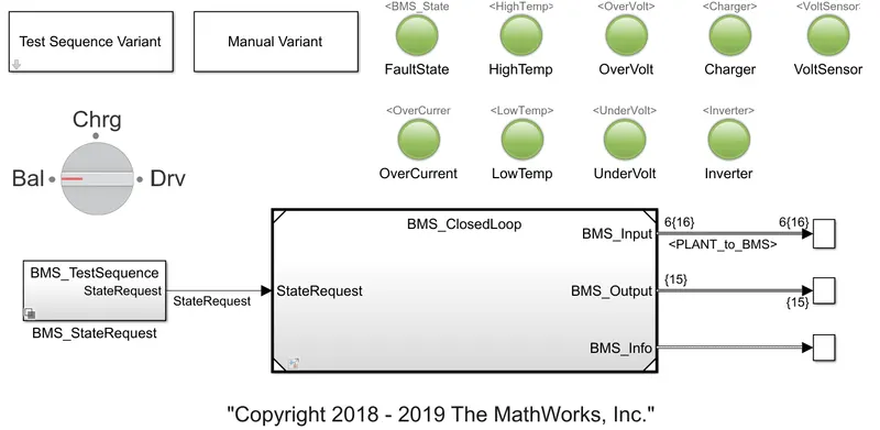
Here after stimulation we can see all the lights have turned green which indicates that there is no fault or errors in the model
RESULT (CASE 1)
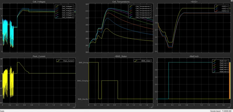
- From the graph we can see that the voltage of cell 1 and cell 2 are different and others lies between them, the highest voltage is for cell 2 and the lowest is for cell 1.
- Hence the cell 1 will control the balancing command of the pack.
- It can be clearly seen from the plot of balancing command, Expect the cell 1 all other cell were balanced passively.
- During the stimulation time from 0 to 3000 seconds the model is in driving mode.
- The voltage and current varies according to the drive load.At this time we can see the cell temperature is raising.Also the SOC dropes from 80% to 45%.
- From 3000 to 4000 seconds the model is in balancing state.The voltage, current,SoC found to be constant and the Temperature was decreasing since no load or charging is done.
- From 4000 to 9000 seconds the model is in charging mode.
- We can observe that the voltage has increased to 3.7v and the current increased nearly 30A and remain some time, whereas the voltage was found to increase rapidly and reach to 4.2 V and remain constant for some time.
- The temperature was found to incerase rapidly at first and then found to decrease slowly.
- The SoC is found to increase from 50% to 100% in 7000 seconds.
- Then from 9000 second onwards the model went to standby state.
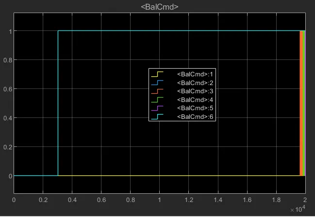
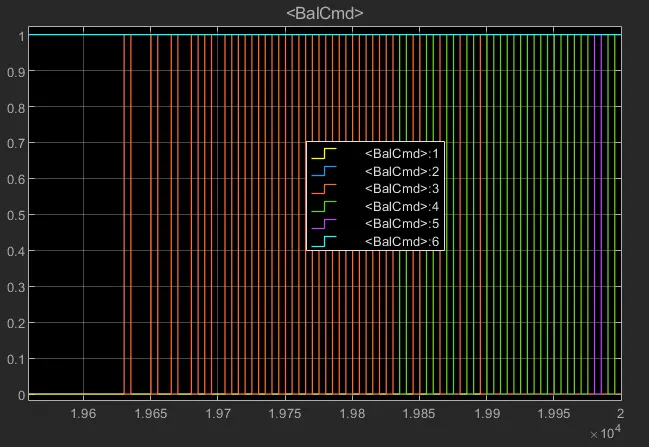
- Here we can see the balancing command of cell 1 is zero and others its 1.It shows expect cell 1 all are passively balanced.
- It is also important to notice at the end of the stimulation at 19000 seconds the balancing command osillates in a pulse form.
- Its because the threshold set in the state flow is so close so that the condition goes form balancing to not balancing so quickly.
- Inorder to solve this porblem the threshold values should be kept by allowing a gap between the values where transition should occure.
Test case 2 Stimulation
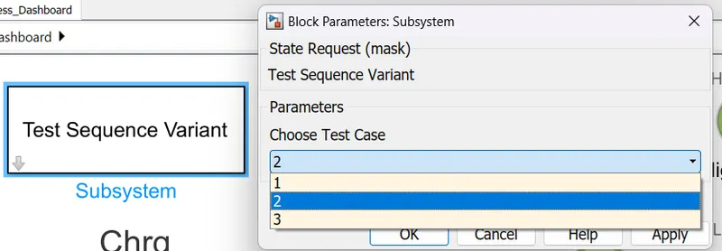
The test case 2 is selected by going to the Test sequence variant block and selecting 2 from the choose test case drop down list.
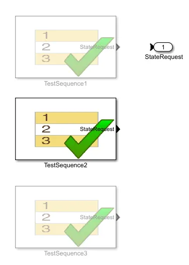

- Now if we check the BMS state request block we can see the sequences and its timing of drivin,charging and standby conditions.
- Here we can see that the Test Sequence 1 has got highlited,it is because we have selected the 1 st test case from the test sequence variant block.
- This will change according to the test case selection automatically.
- When the stimulation starts the model is in driving and after 5000 seconds the state changes to charging.
After simulating the model for 20000 seconds case 2
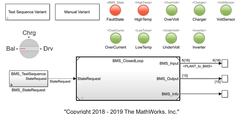
- Here we can see that the BMS system detected the fault in the battery pack and we can understand it by see the red indication
- Also the High temp indicator turned red indicates that the fault is the raise in the battery pack temperature.
RESULT (CASE 2)
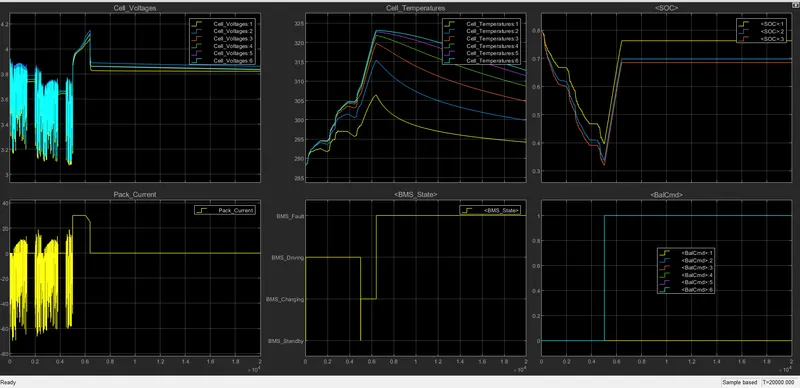
scope during 6400 sec when fault occured
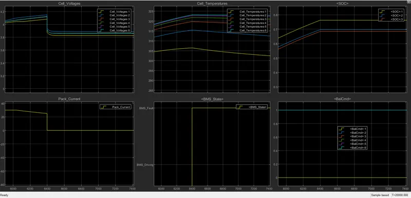
- Here we can see that initially the model is in driving mode for 5000 seconds.
- During this time the SoC was decreased form 80% to 30%. The temperature was also found raising.
- After 5000 second the model switches to charging mode.
- During this time if we look in the temperature graph the temperature raise above 320 which is not normal and at this time the fault signal is activated, which can be seen in the BMS state graph.
- Also the indication was shown in red.
- At this time the SoC was 70% and from that moment the charging was stopped and the SoC stood constant
Test case 3 Stimulation
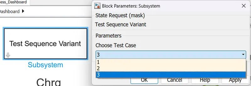
The test case 3 is selected by going to the Test sequence variant block and selecting 3 from the choose test case drop down list.
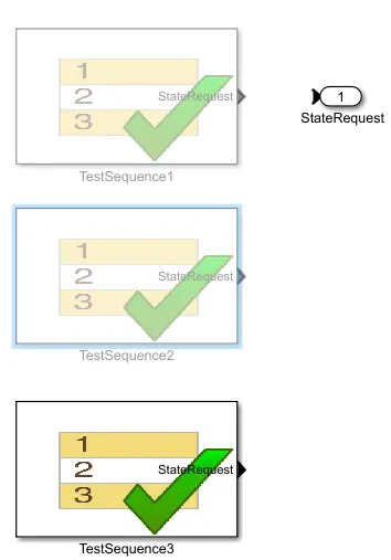
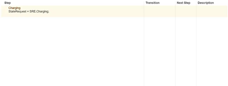
- Here we can see that the Test Sequence 3 has got highlited,it is because we have selected the 3rd test case from the test sequence variant block.
- Here the model is in full time charging only.
After simulating the model for 20000 seconds case 3
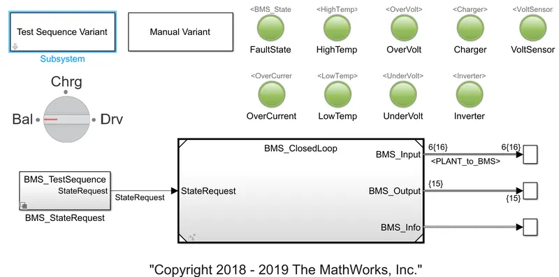
Here after stimulation we can see all the lights have turned green which indicates that there is no fault or errors in the model
RESULT (CASE 3)
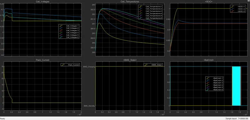
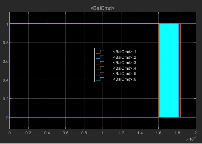
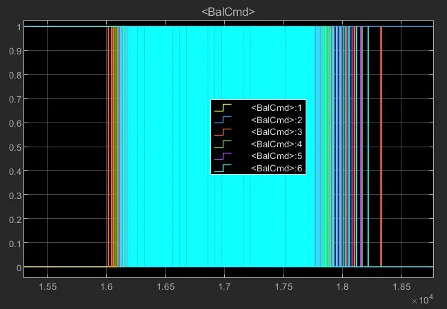
- In case 3 the model is only in charging state.
- The temperature of each cell increases rapidly and then decrease very slowly.
- No fault were found in this stimulation.
2 Coulomb counting
Coulomb counting is a technique used to estimate the amount of charge that has been delivered or removed from a battery by monitoring the flow of electrical current over time. In other words, it is a method of tracking the movement of electrons into or out of a battery, in order to determine the amount of charge that has been transferred.
The process involves measuring the current flowing into or out of the battery over a period of time, and then integrating the current measurement over that time period. This integration gives an estimate of the total charge that has flowed through the system.
Coulomb counting can be used to monitor the state of charge of a battery, and is often used in battery management systems to prevent overcharging or overdischarging of the battery. It is also used in electronic devices to estimate the remaining battery life, by measuring the amount of charge that has been used and comparing it to the total capacity of the battery.
Method of Coulomb counting by BMS
Battery Management Systems (BMS) use Coulomb counting to estimate the State of Charge (SOC) of a battery. The SOC is an important parameter that describes the amount of energy remaining in the battery, relative to its total capacity.
To implement Coulomb counting for SOC estimation, the BMS first measures the current flowing in and out of the battery over a certain period of time. This is typically done using a shunt resistor or a Hall-effect sensor to measure the current, and an Analog-to-Digital Converter (ADC) to convert the analog signal into a digital signal that can be processed by the BMS.
The BMS then integrates the current measurement over time, to estimate the amount of charge that has flowed into or out of the battery during that time period. This charge measurement is then used to update the SOC of the battery.
However, Coulomb counting is not a perfect method, as it can suffer from errors due to factors such as measurement inaccuracies, temperature variations, and changes in battery chemistry over time. To improve the accuracy of Coulomb counting, BMS may use additional methods such as temperature compensation and voltage-based estimations to refine the SOC calculation.
Modified Coulomb Counting Method
The modified Coulomb counting method uses the corrected current to improve the accuracy of estimation.
The corrected current is the function of discharging current. There is a quadratic relationship between the corrected current and discharging current of battery. By practice of experimental data, corrected current is calculated by the following form:
where k2,k1andk0">k2,k1andk0 are constant values obtained from the practice experimental data.
In modified Coulomb counting method, SOC is calculated by the following equation:
The experimental results show that the accuracy of the modified Coulomb counting method is superior to the conventional Coulomb counting method.
But there are several factors that affect the accuracy of Coulomb counting method including temperature, battery history, discharge current, and cycle life.
Closed loop BMS system
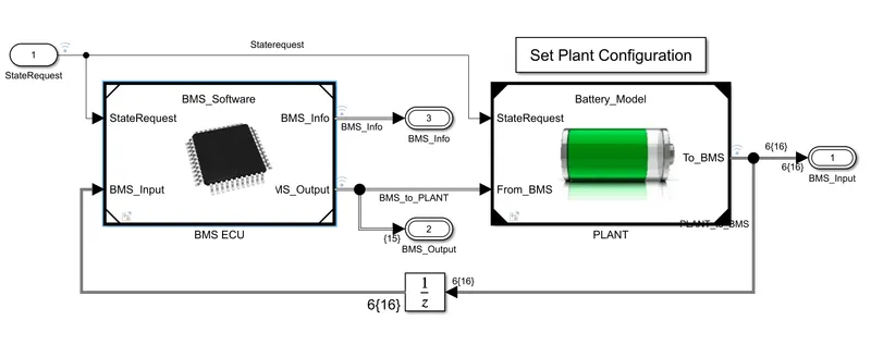
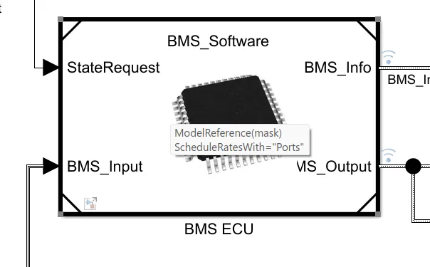
BMS ECU
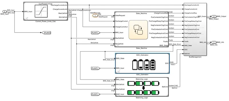
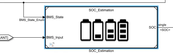
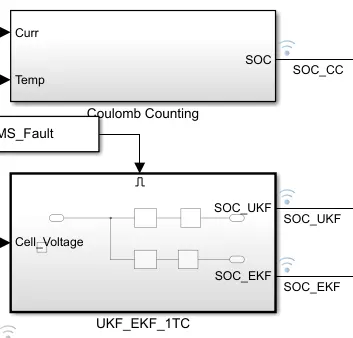
Here inside the SOC estimation we can see there is 3 methods of estimation used: Columb counting, Unscented Kalman Filter (UKF) and Extended Kalman Filter (EKF).
Columb counting
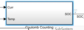
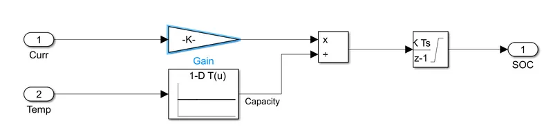
- Temperature and current are taken as input.
- The current signal is given to the gain block and the temperature is given to capacity as it varies according to the temperature.
- These inputs are given to integration where current will be integrated wrt time.
- This output is given to another block where it is divided by capacity and henceforth the SOC is estimated.
- The accuracy of coulomb counting is less and also it has some disadvantages
- One of the disadvantage of coulomb counting is that it is sensitive to initial SoC and another disadvantage is that any error in the measurement of current value will keep on adding during it is integrated.
CONCLUSION
- Stimulated 3 test cases from harness dashboard and studied the results in detail.
- Studied about coulomb counting and how BMS implements coulomb counting for SOC estimation
REFERENCE