Week 4.1 - Genetic Algorithm
AIM
To write a code in MATLAB to optimise the stalagmite function and find the global maxima of the function using Genetic Algorithm.
Theory
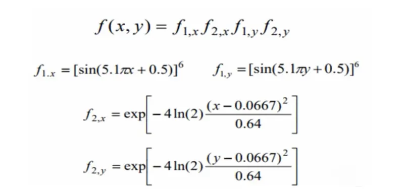
Stalagmite Function:
A stalagmite function generally refers to the function with which we are generating values over a stalagmite kind of surface for finding out the local and global maxima and minima of that particular given function.
Genetic Algorithm :
Genetic Algorithm (GA) is a branch of field of study called evolutionary comutation. It is based on evolution theory by Darwin. GA is used to optimize a given function to find its maximum or minimum value. The basic components of a GA are
1. Fitness function : It is the function that GA is trying to optimize.
2. A population of chromosome : It is the numerical values that represent all the solutions to the function. The selection operator chooses some of the chromosomes (with replacement) for reproduction based on probability distribution. fitter the chromosome more likely it is to be selected.
3. Cross over : This operator swaps in random a subsequence of two of the chosen chromosomes to create two offspring. Usually each chromosome is converted into binary code and then cross over is done from one parent chromosome into another.
4. Mutation : Mutation operator randomly flips individual bits in the new chromosomes.
The GA syntax in Matlab is given by :
x = ga(fun,nvars,A,b,Aeq,beq,lb,ub)
x = ga(fun,nvars,A,b,Aeq,beq,lb,ub,nonlcon)
x = ga(fun,nvars,A,b,Aeq,beq,lb,ub,nonlcon,options)
x = ga(fun,nvars,A,b,[],[],lb,ub,nonlcon,IntCon)
x = ga(fun,nvars,A,b,[],[],lb,ub,nonlcon,IntCon,options)
[x,fval,exitflag,output] = ga(___)
[x,fval,exitflag,output,population,scores] = ga(___)
Where,
fun = objective function
nvars = number of design variables
A and B = subject to linear inequalities of the form A*x <=B
Aeq and Beq = subject to linear equalities of the form A*x = B
LB = lower bound
UB = upper bound
nonlcon = non linear inequalities
intcon = integer constrained
options = helps to add contraint tolerance by increasing the population size
Description
x = ga(fun,nvars) finds a local unconstrained minimum, x, to the objective function, fun. nvars is the dimension (number of design variables) of fun.
x = ga(fun,nvars,A,b) finds a local minimum x to fun, subject to the linear inequalities A*x ≤ b. ga evaluates the matrix product A*x as if x is transposed (A*x').
x = ga(fun,nvars,A,b,Aeq,beq) finds a local minimum x to fun, subject to the linear equalities Aeq*x = beq and A*x ≤ b. (Set A=[] and b=[] if no linear inequalities exist.) ga evaluates the matrix product Aeq*x as if x is transposed (Aeq*x').
x = ga(fun,nvars,A,b,Aeq,beq,lb,ub) defines a set of lower and upper bounds on the design variables, x, so that a solution is found in the range lb ≤ x ≤ ub. (Set Aeq=[] and beq=[] if no linear equalities exist.)
x = ga(fun,nvars,A,b,Aeq,beq,lb,ub,nonlcon) subjects the minimization to the constraints defined in nonlcon. The function nonlcon accepts x and returns vectors C and Ceq, representing the nonlinear inequalities and equalities respectively. ga minimizes the fun such that C(x) ≤ 0 and Ceq(x) = 0. (Set lb=[] and ub=[] if no bounds exist.)
x = ga(fun,nvars,A,b,Aeq,beq,lb,ub,nonlcon,options) minimizes with the default optimization parameters replaced by values in options. (Set nonlcon=[] if no nonlinear constraints exist.) Create options using optimoptions.
x = ga(fun,nvars,A,b,[],[],lb,ub,nonlcon,IntCon) or x = ga(fun,nvars,A,b,[],[],lb,ub,nonlcon,IntCon,options) requires that the variables listed in IntCon take integer values.
x = ga(problem) finds the minimum for problem, a structure described in problem.
[x,fval] = ga(___), for any previous input arguments, also returns fval, the value of the fitness function at x.
[x,fval,exitflag,output] = ga(___) also returns exitflag, an integer identifying the reason the algorithm terminated, and output, a structure that contains output from each generation and other information about the performance of the algorithm.
[x,fval,exitflag,output,population,scores] = ga(___) also returns a matrix population, whose rows are the final population, and a vector scores, the scores of the final population.
Here is how a genetic algorithms works
-
The algorithm begins by creating a random initial population.
- The algorithm then creates a sequence of new populations. At each step, the algorithm uses the individuals in the current generation to create the next population. To create the new population, the algorithm performs the following steps:
- scores each member of the current population by computing its fitness value. These values are called the raw fitness scores.
- scales the raw fitness scores to convert them into a more usable range of values. These scaled values are called expectation values.
- Selects members, called parents, based on their expectation.
- Some of the individuals in the current population that have lower fitness are chosen as elite. These elite individuals are passed to the next population.
- Produces children from the parents. Children are produced either by making random changes to a single parent—mutation—or by combining the vector entries of a pair of parents—crossover.
- Replaces the current population with the children to form the next generation.
3. The algorithm stops when one of the stopping criteria is met
4. The algorithm takes modified steps for linear and integer constraints.
5. The algorithm is further modified for nonlinear constraints.
Some advantages of genetic algorithms this method are the following:
1) They usually perform better than traditional feature selection techniques.
2) Genetic algorithms can manage data sets with many features.
3) They don't need specific knowledge about the problem under study.
4) These algorithms can be easily paralelized in computer clusters.
Program code
Stalagmite function code used
%stalagmite function
function [f] = stalagmite(input_vector)
 x=input_vector(1);
 y=input_vector(2);

 f1x = (sin(5.1*pi*x+0.5)).^6;
 f1y = (sin(5.1*pi*y+0.5)).^6;
 f2x = exp((-4*log(2))*((x-0.0667).^2/0.64));
 f2y = exp((-4*log(2))*((y-0.0667).^2/0.64));
 f = -f1x*f1y*f2x*f2y;
end
Function code Explaination
- The function used here is for calculating the stalatmite function.
- This function will create the data for the plot , ie. the data required for genetic algorithm to perform on to find the global maxima.
- The name of the function is stalagmite(), which takes in the input column vectors.
- The first column and the second column vectors are seperated into x & y.
- The the values of stalagmite function is calculated numerically.
- NB: The '-ve' sign is given at the end, since the stalagmite function will calculate the global minma but we are interested in finding global maxima.
- Otherwise if we didn't put the '-ve', while ploting we will get the plot of stalagmites hanging downward.
- The function will return the data for creating stalagmite plot.
- Main function
close all
clear all
clc

% Defining serch space
x = linspace(0,0.6,150);
y = linspace(0,0.6,150);
num_case = 50;

% Creating 2D mesh
[xx yy] = meshgrid(x,y);

% Evaulating the stalagmite function
for i = 1:length(xx)
     for j = 1:length(yy)
         input_vector(1) = xx(i,j);
         input_vector(2) = yy(i,j);
         f(i,j) = stalagmite(input_vector);
     end
end

% Study1 statistical behaviour
tic
for i = 1:num_case
    [input,fval(i)] = ga(@stalagmite,2); % basic ga() function
    xopt(i)= input(1);               % optimum value of x at each iteration
    yopt(i)= input(2);               % optimum value of y at each iteration
end
study1_time = toc

figure(1)
subplot(2,1,1);
hold on
surf(x,y,-f);
shading interp
plot3(xopt,yopt,-fval,'Marker','o','MarkerSize',5,'markerfacecolor','g');
title('ga with Unbounded inputs');
xlabel('x inputs');
ylabel('y inputs');
zlabel('z axis');
grid on

subplot(2,1,2);
plot(-fval);
xlabel('Iteration');
ylabel('Function Maxima');
grid on

% Study 2 ga with Upper and Lower bound
UB = [0.6,0.6];
LB = [0,0];
tic
for i = 1:num_case
    [input,fval(i)] = ga(@stalagmite,2,[],[],[],[],LB,UB); % ga() function with UB & LB
    xopt(i)= input(1);               % optimum value of x at each iteration
    yopt(i)= input(2);               % optimum value of y at each iteration
end
study2_time = toc

figure(2)
subplot(2,1,1);
hold on
surf(x,y,-f);
shading interp
plot3(xopt,yopt,-fval,'Marker','o','MarkerSize',5,'markerfacecolor','g');
title('ga with Bounded inputs');
xlabel('x inputs');
ylabel('y inputs');
zlabel('z axis');
grid on

subplot(2,1,2);
plot(-fval);
xlabel('Iteration');
ylabel('Function Maxima');
grid on

% Study 3 - ga with optimization option
tic
options = optimoptions('ga');
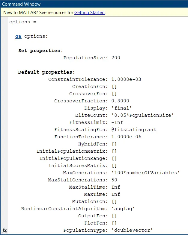
options = optimoptions(options,'PopulationSize',200)
for i = 1:150
    [input,fval(i)] = ga(@stalagmite,2,[],[],[],[],LB,UB,[],[],options); % ga() function with UB & LB & optimization options
    xopt(i)= input(1);               % optimum value of x at each iteration
    yopt(i)= input(2);               % optimum value of y at each iteration
end
study3_time = toc

figure(3)
subplot(2,1,1);
hold on
surf(x,y,-f);
shading interp
plot3(xopt,yopt,-fval,'Marker','o','MarkerSize',5,'markerfacecolor','g');
title('ga with Bounded inputs & optimization option');
xlabel('x inputs');
ylabel('y inputs');
zlabel('z axis');
grid on

subplot(2,1,2);
plot(-fval);
xlabel('Iteration');
ylabel('Function Maxima');
grid on
Program Explaination
- The code begins with closing & clearing the memory using close all, clear all clc functions.
- Two one dimensional arrays x & y were created using linespace(), which will be the serch space for the genetic algorithem to find the maxima
- A variable called num_case is defined and initlized to 50, this is for running the genetic algorithm for 50 times.
- A 2D mesh is created using the meshgrid() function and the value is stored to xx & yy.
- The next step is evaulating stalagmite function.
- Since the input for stalagmite function requires 2 variables the matrix xx & yy is combined into a colum matrix which have 150 rows and 2 columns using nested for loop.
- The stalagmite function is called inside the loop itslef so that the each value of stalagmite function after calculation can be saved into matrix f[150*150].
Next is the statistical study of ga()
- In the first study the optimization solver ga() is used with mandatory inputs only no additional information were provided.
- The basic genetic algorithm syntax is ga(@function name,number of variables).
- To calculate the time required for excuitng the study1 time counting function tic is used this command will start the timer.
- The genetic algorithm is called by passing the funtion handle stalagmite and the number of variables used in the function.
- Using the for loop the genetic algorithm is made to run for 50 times.
- Each optimum value and corresponding value of x & y were made to store in fval and input.
- After the end the time taken is calculated using the toc function and is stored into study1_time.
- figure(1) command is used to getting the first figure.
- subplot() command is used for ploting two plot in same figure.
- The 3D representation is made using the surf() command.
- In the surf() command the value of 'f' has given -ve sign this is for getting the Global maxima .
- shading interp will turn off the grid formation over the stalagmite function plot.
- plot3() command is used for creating a 3D plot which has 3 axis x,y&z. It is also important to give the fval a -ve sign for getting the global maxima.
- The title,labeling of axis and showing grid were done using the following commands title(), xlabel(), ylabel(), zlabel() & grid on respectively.
- The to see the optimum value ga created on each iteration subplot() with plot() is used. This graph will show the value of maxima that the ga() generated on each iteration.
- The labeling were done using xlabel() and ylabel(), also the grid is set on by grid on.
The Study2 of ga by defining the limits.
- Since the ga starts form random sampling the starting points are scattered all over the place.So in study 2 the limits within which the serch has to be done is initilized.
- The limits are set using UB (upper bound) & LB(lower bound).
- The ga() function will change from basic to more specific as ga(@stalagmite,2,[],[],[],[],LB,UB).
- Expect the change in ga() function all other code is same as study 1
The study3 of ga function by increasing the population (options)
- The ga() function is again modified to get more optimum result.
- In the ga function one option is added ie the population size and the ga function will become ga(@stalagmite,2,[],[],[],[],LB,UB,[],[],options).
- The population size was set to 200
- Expect the change in ga() function all other code is same as study 1
Conclusion
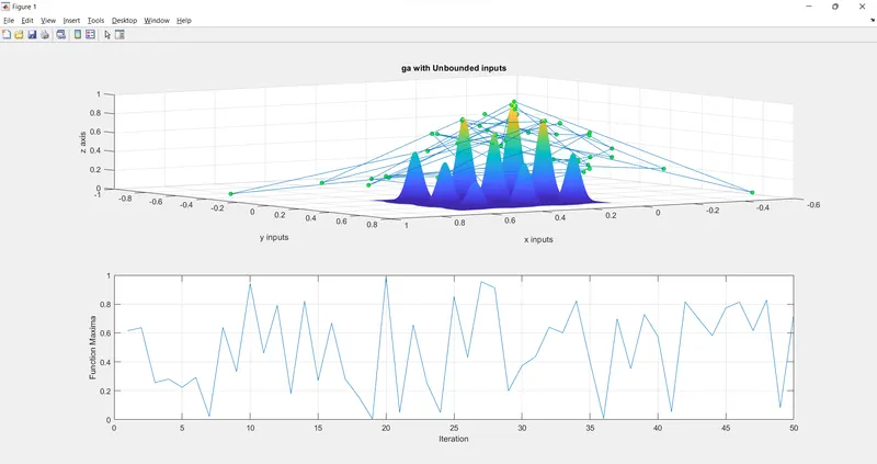
Study 1
- It is already known that the genetic algorith will find the global minima by sampling random variables.
- The ga was stating points that are too far from the stalagmites.
- The results show the ga was giving the value of maxima randomly and has a huge variation on each time of program excuation.
- It is not all predicting the global maxima accuratly.
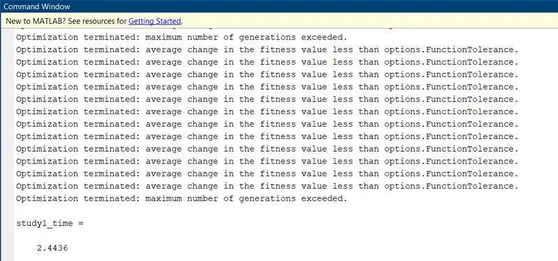
- Time taken to excuite code is 2.44 sec.
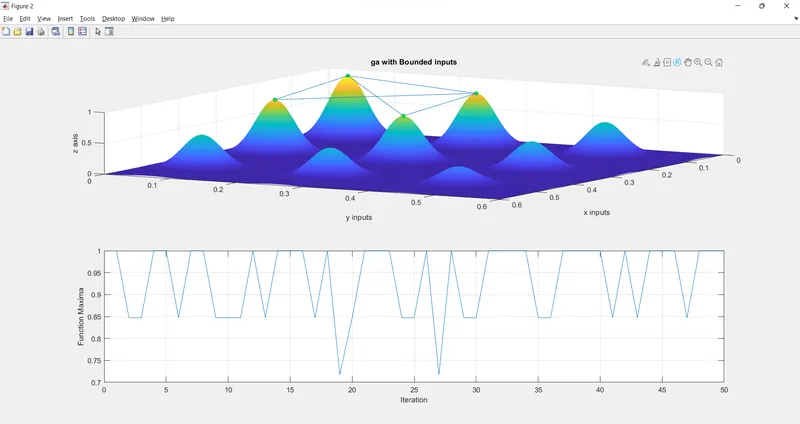
Study 2
- After modefying the ga() giving the limits within which the functuion has to serch for maxima, the output were little more narrowed down and also the bouncing of maxima was slightly decreased.
- The consistacy of giving the maxima is better than the study1 but still the maxima has not accuratly predicted.
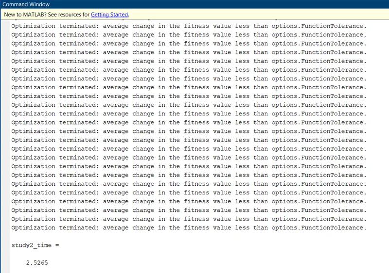
- Time taken to excuite code is 2.52 sec.
Study 3
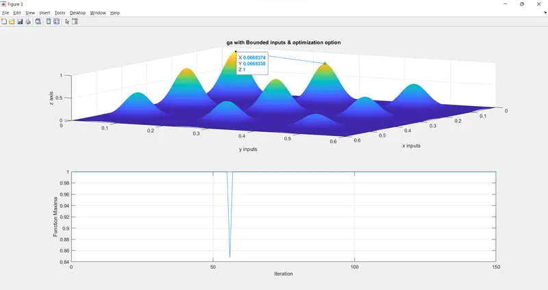
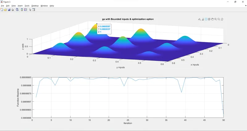
- In the third study the ga() is again modified by increasing the size of population along with providing the boundry limits.
- The modification provided much better results.The ga() has predicted the global maxima accurately most of all the times
- In the first run the subplot showed that only one time the ga predicted different value but the prediced maxima was not too far.
- In the second run the subplot showed that the ga is predicting the global maxima with slight variation which is negligibly small with high precision.
- In all the time the ga() predicts the global maxima = 1
- at x = 0.066832
- at y = 0.066833
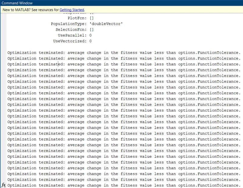
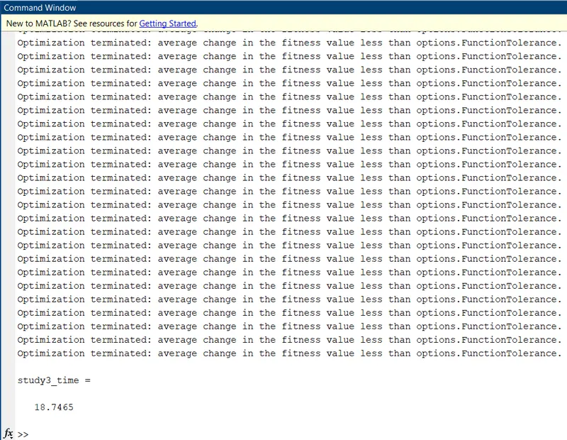
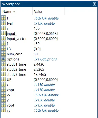
- Each time further addition of optimization parameters to ga() is making the code slower. it took 18.74 sec to run the function.
Outputs
1. Study 1 - ga() without bounded inputs :
Command window
2. Study 2 - ga() with bounded inputs
Command Window
3 Study 3 - ga() with options(Population size)
After running the code for first time:
After running the code for second time:
Command Window
Workspace
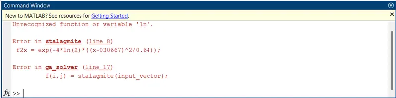
Error Encountered
Used ln instead of log
Reference
https://in.mathworks.com/help/gads/how-the-genetic-algorithm-works.html