Week 3 - Solving second order ODEs

AIM

1. To write a program code to solve the ODE which represents the equation of motion of a simple pendulum.
2. To create the animation of movement of the simple pendulum with damping w.r.t time.

Theory

• The motion of a simple pendulum is a basic example of simple harmonic motion.
• The system consisting of a small bob and a massless string. Movement of the pendulum depends on Newton's second law.
• When this law is written down, a second-order Ordinary Differential Equation is formed that describes the position of the end of the pendulum w.r.t time.

Free body diagram of simple pendululm :

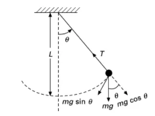
The above figure shows an idealized pendulum, with a "massless" string or rod of length L and a bob of mass m.When the bob is moved from its rest position and let go, it swings back and forth. The time it takes the pendulum to swing from its farthest right position to its farthest left position and back to its next farthest right position is the period of the pendulum.

The primary forces acting on the bob are the gravitational force that makes it move in the first place and the force exerted by the string to keep it moving along a circular path. In addition, there may be a damping force from friction at the pivot or air resistance or both.

An ordinary differential equation (ODE) is a differential equation containing one or more functions of one independent variable and the derivatives of those functions. The ODE equation and the calculations are shown below

The equation of motion of a simple pendulum with damping:

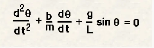
In the above equation,

g = 9.81 (gravity in m/s^2)

L = 1 (length of the pendulum in m)

m = 1 (mass of the ball in kg)

b = 0.05 (damping coefficient.)

Program Code

%Second_order_ODE_solving
close all
clear all
clc

%constants
b=0.05;
l=1;
g=9.81;
m=0.1;

%initial condition
theta_0 = [0,3];

%time points
t_span = linspace(0,20,500);

%solving ODE
[t,result] = ode45(@(t,theta) ode_fun(t,theta,b,l,g,m),t_span,theta_0);

%plotting displacement & velocity w.r.t time
figure(1)
hold on
plot(t,result(:,1))
plot(t,result(:,2))
title('SHM of simple pendulum with Damping')
xlabel('Time (seconds)')
ylabel('Displacement & Velocity')
legend('Displacement','Velocity')
grid on
hold off

%Pendulum movement stimulation
ct=1;
for i = 1:length(result(:,1))
    x_start=0;
    y_start=0;
    x_end = l*sin(result(i,1));
    y_end = -l*cos(result(i,1));
    figure(2) 
    plot([-0.6,0.6],[0,0],'linewidth',4,'Color','black')
    line([0,0],[0.5,-1.3],'LineStyle','- -','Color','black','lineWidth',1.5)
    hold on
    text(0.2,0.5,sprintf('Displacement = %f',result(i,1)),"EdgeColor",'r')
    text(0.2,0.3,sprintf('Velocity = %f',result(i,2)),"EdgeColor",'r')
    plot([x_start,x_end],[y_start,y_end],x_end,y_end,'b.','MarkerSize',60,'LineWidth',2)
    axis([-1,1,-1.5,1])
    title('Simple pendulum stimulation with damping')
    grid on
    pause(0.03);
    hold off
    M(ct) = getframe(gcf);
    ct=ct+1;
end
movie(M);
bob_mov = VideoWriter('Pendulum stimulation','Uncompressed AVI');
open(bob_mov);
writeVideo(bob_mov,M);
close(bob_mov);

Function code used

%ode_fun
function [dtheta_dt] = ode_fun(t,theta,b,l,g,m)
  theta1 = theta(1);
  theta2 = theta(2);
  dtheta1_dt = theta2;
  dtheta2_dt = -(b/m)*theta2-(g/l)*sin(theta1);
  [dtheta_dt] = [dtheta1_dt;dtheta2_dt];
end 

Program Explaination

• First of all the memory and storages are cleared using the close all,clear all and clc functions.
• The constants b,l,g,m are initilized.
• The initial condition of the bob with angular displacement '0' & anglular veloctity 3 rad/sec was defined and assigned to 'theta_0'.
• The integration limits of time was defined from 0 second to 20 second and is equally divided for 500 intervals using the function linspace() and the vector is assigned to t_span.
• To solve the second order ODE the function ode45() is used.
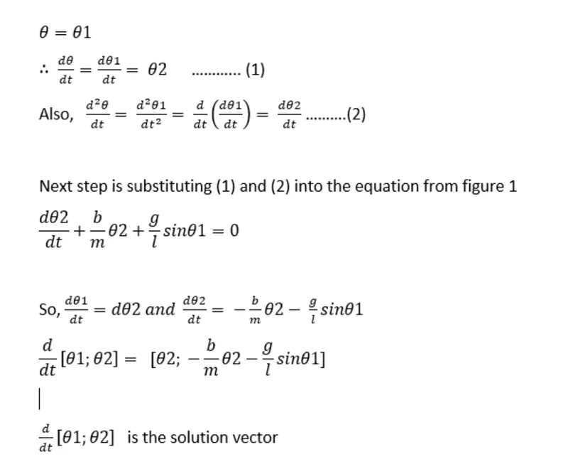
• The user defined function ode_fun() is used to solve the second oder ODE by breaking down on to two first order ODEs
• The function ode_fun() returns the value of dtheta/dt [dtheta1/dt ; dtheta2/dt] in 2 column vectors.
• The ode45() function is dependent on time and angle theta, hence the time limit is provided by t_span & the intial conditions were provided by theta_0.
• After solving the second order ODE the results were assigned to the vector [t ,result].
• The result vector obtained contains the angular displacement and angular velocity w.r.t time.
• To plot the angular displacement and angular velocity against time with damping figure() command is used.Using hold on command both displacement and velocity is ploted on same graph.
• plot(t,result(:,1)) is used to plot the angular displacement against time and plot(t,result(:,2)) is used to plot angular velocity against time.

Result

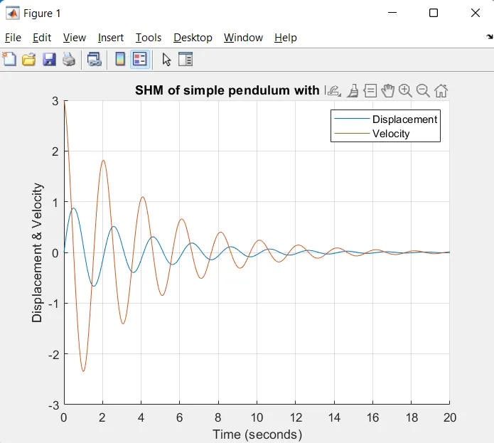
• The second order ODE of simple pendulum is solved and graph have been ploted for Displacement & Velocity against time.
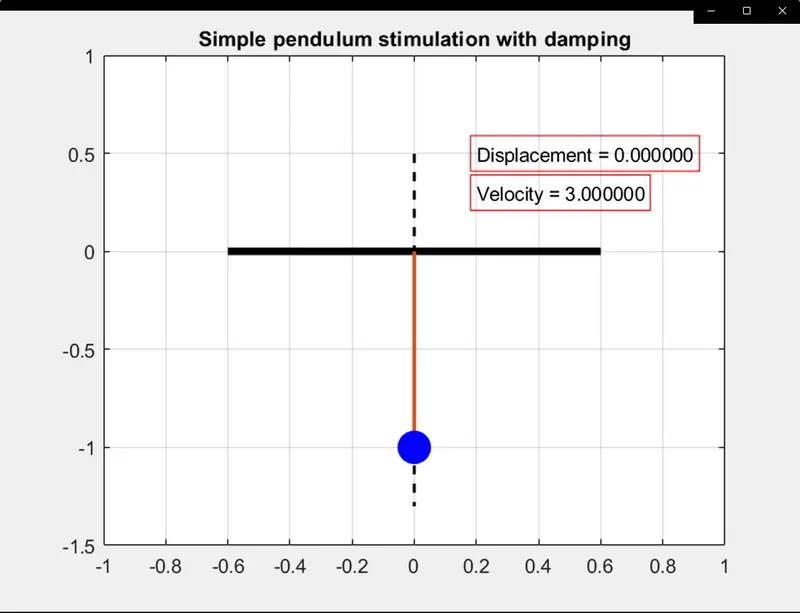
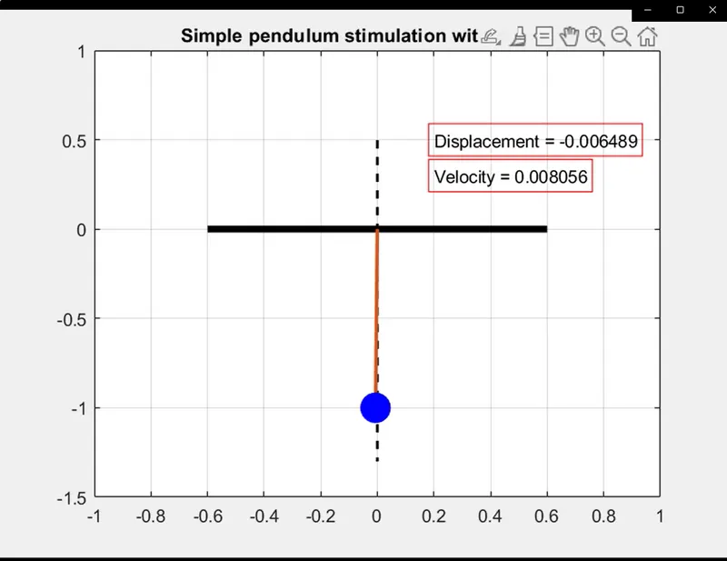
• The motion of simple pendulum with damping is stimulated for 20 second.

The below figure is the plot of Displacement & Velocity of bob of pendulum againt time for 20 seconds.

The below figures shows the starting and ending of the stimulation of motion of simple pendulum respectively:

Video link :

https://youtu.be/j02QpMj55Jc

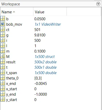
Workspace

References

https://in.mathworks.com/matlabcentral/answers/31568-printing-value-of-a-variable-in-a-plot-at-some-fixed-coordinates

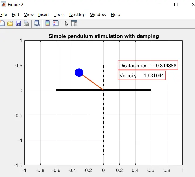
Error encountered

The stimulation went wrong

Error Clearing