Project 2 - Rankine cycle Simulator
AIM
- To Simulate a Rankine cycle using matlab.
- Extracting Steam and water properties from XSteam data.
- Calculating all the state points of the cycle based on User inputs.
- Plotting the T vs s and H vs s plot for the given input.
Theory
Rankine cycle is the theoretical cycle on which the steam turbine (or engine) works.
The Rankine cycle is an idealized thermodynamics cylce describing the process by which certain heat engines, such as steam turbine or reciprocating steam engines, allow mechanical work to be extracted from a fluid as it moves between a heat source and heat sink. The Rankine cycle is named after William John Macquorn Rankine, a Scottish polymath professor at Glasgow University.
Heat energy is supplied to the system via a boiler where the working fluid (typically water) is converted to a high pressure gaseous state (steam) in order to turn a turbine. After passing over the turbine the fluid is allowed to condense back into a liquid state as waste heat energy is rejected before being returned to boiler, completing the cycle. Friction losses throughout the system are often neglected for the purpose of simplifying calculations as such losses are usually much less significant than thermodynamic losses, especially in larger systems.
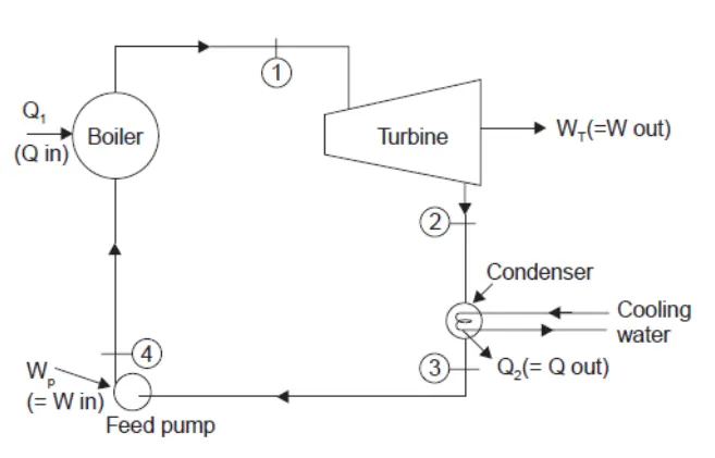
- Four components of the Rankine cycle:
- Pump
- Boiler
- Turbine
- Condenser
-
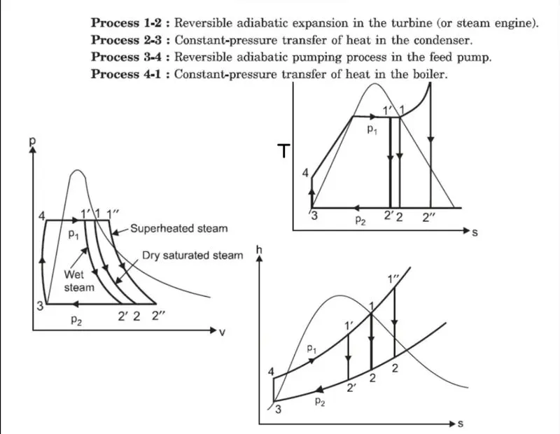
- Four processes of the Rankine cycle:
1 - 2: Isentropic Expansion
Superheated steam enters into the Turbine and expands isentropically resulting in the production of work. The shaft of the turbine is connected to the generator. This results in the production of electricity i.e Mechanical energy gets converted into electric energy. Work produced by the turbine,

- Depending on exit state of turbine (superheated state, saturated vapor state or liquid-vapor mix state), the values of enthalpy are calculated and using entropy relation between states 1 and 2, dryness fraction is calculated.
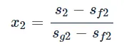
- If State 2 is in saturated or liquid-vapor mix state then enthalpy at state 2 is given by

- If State 2 is in superheated state the enthalpy at state 2 is given by,

where,
T2 - Temperature at state 2
 - Saturation temperature at P2
 - enthalpy and entropy at saturated liquid state.
 - enthalpy and entropy at saturated vapor state.
 - Specific heat of liquid vapour
2-3: Constant Pressure Heat RejectionThe expanded vapour is then passed through a condenser, where it gets condensed and converts into liquid again. This liquid is again pumped to the boiler.
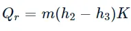
Process 2-3 may contain 2 regions depending on exit state of turbine.
- If end state 2 is in superheated region then the process contains 2 regions. Superheated region from state 2 to saturated vapor state on pressure P2 which is a curve outside saturation curve and Phase change region from saturated vapor state on pressure P2 to State 3 which is a straight line inside saturation curve.
- If end state 2 is in saturated region or liquid-vapor mix region then the process contains only phase change region from saturated vapor state on pressure P2 to State 3 which is a straight line inside saturation curve.
3-4: Isentropic Compression by the Pump
The water enters into the pump in a saturated state. Then the liquid is compressed isentropically until it meets the boiler pressure. Work done by the pump is,

4-1: Constant Pressure Heat Addition
Boiler (4-1): The water enters into the boiler as compressed and leaves as superheated from the boiler. Thus the phase changes from liquid to vapour. The heat supplied by the boiler is

Process 4-1 contains 3 regions i.e, Subcooling, Phase change and Superheating.
- Subcooling Region: From state 4 to saturated liquid state on pressure P1 . It is a curve along constant pressure.
- Phase Change Region: From saturated liquid state on pressure P1 to saturated vapor state on pressure P1. It is straight line inside saturation curve at constant pressure.
- Superheat Region: From saturated vapor state on pressure P1to State 1. It is a curve along constant pressure.
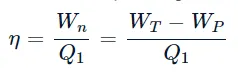
The efficiency of the Steam Cycle is given by

PROGRAM CODE
%Rankine_cylce_stimulator
close all
clear all
clc

%inputs
fprintf('\n                   Rankine Cycle Stimulator           \n')
fprintf('\n\nProcess 1-2: Isentrophic Expansion in Turbine.')
fprintf('\nProcess 2-3: Constant Pressure Heat rejectioin in Condensor.')
fprintf('\nProcess 3-4: Isentropic Compression by Feed Pump.')
fprintf('\nProcess 4-1: Constant Pressure Heat addition in Boiler.\n')
p1=input('\nEnter the Pressure at Turbine inlet(in bars) : ');
t1=input('Enter the Temperature at Turbine inlet(in Degree Celcius) : ');
p2=input('Enter the Pressure at Condensor inlet (in bar) : ');

%calculation
p4=p1;   %constant pressure heat addition
p3=p2;   %constant pressure heat rejection

%extracting state point 1 data
h1=XSteam('h_pT',p1,t1);   %enthalpy at pressure p1&t1
s1=XSteam('s_pT',p1,t1);   %endropy at pressure p1&t1

%extracting state point 2 data
s2=s1;                     %isentrophic expansion
sf2=XSteam('sL_p',p2);     %saturated liquid endropy at p2
sg2=XSteam('sV_p',p2);     %saturated vapour endropy at p2
hf2=XSteam('hL_p',p2);     %saturated liquid enthalpy at p2
hg2=XSteam('hV_p',p2);     %saturated vapour enthalpy at p2
x2=((s2-sf2)/(sg2-sf2));   %vapour fraction
if x2<=1                   %point either in liquid-vapour or saturated vapour
    h2=hf2+(x2*(hg2-hf2)); %enthalpy at point2 (hfg2=hg2-hf2)
    t2=XSteam('T_ph',p2,h2);
else                       %point 2 at superheated region(x2>1)
    tsat_p2=XSteam('Tsat_p',p2);
    t2=XSteam('T_ps',p2,s2);
    Cpv=XSteam('Cp_pT',p2,t2);
    h2=hg2+(Cpv*(t2-tsat_p2));
end
%extracting state point 3 data
h3=XSteam('hL_p',p3);      %saturated liquid enthalpy at p3
s3=XSteam('sL_p',p3);      %saturated liquid endropy at p3
v3=XSteam('vL_p',p3);      %volume of liquid at p3
t3=XSteam('Tsat_p',p3);    %saturation temperature at p3

%extracting state point 4 data
s4=s3;                     %isentrophic compression
h4=XSteam('h_ps',p4,s4);
t4=XSteam('T_ph',p4,h4);
WP = v3*(p4-p3)*100;

%temperature,endropy & endropy during constant pressure heat addition
t6=XSteam('Tsat_p',p1); %saturated Temperature at  p1
t5=t6;
s5=XSteam('sL_p',p1);   %saturated Liquid entropy at p1
s6=XSteam('sV_p',p1);   %saturated Vapour entropy at p1
h5=XSteam('hL_p',p1);   %saturated Liquid Enthalpy at p1
h6=XSteam('hV_p',p1);   %saturated Vapour Enthalpy at p1

%efficiency
WT=h1-h2;
Wnet=WT-WP;
Qin=h1-h4;
Qout=h2-h3;
NTherm=Wnet/Qin;
SSC=3600/Wnet; %Specific steam consumption
Back_work_ratio = WP/WT;

%Result printing
fprintf('\n****************************************************************\n');
fprintf('                           RESULTS                      \n');
fprintf('\nAt state point 1:');
fprintf('\t\t\t\t\t\tAt state point 2:\n');
fprintf(' P1 is : %4.2f Bar',p1);
fprintf('\t\t\t\t\t\t P2 is : %4.2f Bar\n',p2);
fprintf(' T1 is : %4.2f Celcius',t1);
fprintf('\t\t\t\t\t T2 is : %4.2f Celcius\n',t2);
fprintf(' H1 is : %4.2f KJ/Kg',h1);
fprintf('\t\t\t\t\t H2 is : %4.2f KJ/Kg\n',h2);
fprintf(' S1 is : %4.2f KJ/KgK',s1);
fprintf('\t\t\t\t\t S2 is : %4.2f KJ/KgK\n',s2);

fprintf('\nAt state point 3:');
fprintf('\t\t\t\t\t\tAt state point 4:\n');
fprintf(' P3 is : %4.2f Bar',p3);
fprintf('\t\t\t\t\t\t P4 is : %4.2f Bar\n',p4);
fprintf(' T3 is : %4.2f Celcius',t3);
fprintf('\t\t\t\t\t T4 is : %4.2f Celcius\n',t4);
fprintf(' H3 is : %4.2f KJ/Kg',h3);
fprintf('\t\t\t\t\t H4 is : %4.2f KJ/Kg\n',h4);
fprintf(' S3 is : %4.2f KJ/KgK',s3);
fprintf('\t\t\t\t\t S4 is : %4.2f KJ/KgK\n',s4);

%Perfomances
fprintf('\nWork done by Turbine Wt is : %4.2f KJ/Kg',WT);
fprintf('\nWork done by Pump Wp is : %4.2f KJ/Kg',WP);
fprintf('\nNet Work done Wnet is : %4.2f KJ/Kg',Wnet);
fprintf('\nSpecific Steam Consumption [SSC] is : %4.2f Kg/KWh',SSC);
fprintf('\nThermal efficiency Ntherm is : %4.2f percentage',NTherm);
fprintf('\nBack Work Ratio is : %4.4f\n',Back_work_ratio);
fprintf('\n****************************************************************\n');

%Plotting

%Saturation curve of water
Trange=linspace(0,374,500);
for i=1:length(Trange);
    sf(i)=XSteam('sL_T',Trange(i));  % Saturated Liquid Entropy
    hf(i)=XSteam('hL_T',Trange(i));  % Saturated Liquid Enthalpy
    sg(i)=XSteam('sV_T',Trange(i));  % Saturated Vapour Entropy
    hg(i)=XSteam('hV_T',Trange(i));  % Saturated Vapour Entropy
end

%plot for T-S Diagram
figure(1)
hold on
plot(sf,Trange,'--','LineWidth',2,'color','0.2 0.5 1');
plot(sg,Trange,'--','LineWidth',2,'color','0.2 0.5 1');

plot([s1 s2],[t1 t2],[s3 s4],[t3 t4],[s5 s6],[t5 t6],'LineWidth',2,'color','0.2 0.8 0.5');

if x2<=1  %if dryness fraction less than 1 then it will be in liquid vapour mix region
    plot([s2 s3],[t2 t3],'LineWidth',2,'color','0.2 0.8 0.5');%straight line plot
else   %phase change from superheated vapour to saturated liquid
    S2super=linspace(s2,sg2,100);%calculating values of T & H
    for i=1:length(S2super);
        TSuper(i)=XSteam('T_ps',p2,S2super(i));
        HSuper(i)=XSteam('h_ps',p2,S2super(i));
    end
    plot(S2super,TSuper,'LineWidth',2,'color','0.2 0.8 0.5');%curve plot
    plot([sg2 s3],[tsat_p2 t3],'LineWidth',2,'color','0.2 0.8 0.5');
end

SLrange=linspace(s4,s5,500);        %subcooled endropy range
SVrange=linspace(s6,s1,500);        %superheated endropy range
for j=1:length(SLrange)             %T & H range at subcooled region
    TLrange(j)=XSteam('T_ps',p4,SLrange(j));
    HLrange(j)=XSteam('h_ps',p4,SLrange(j));
end
for k=1:length(SVrange)             %T & H range at superheated region
    TVrange(k)=XSteam('T_ps',p1,SVrange(k));
    HVrange(k)=XSteam('h_ps',p1,SVrange(k));
end
plot(SLrange,TLrange,'LineWidth',2,'color','0.2 0.8 0.5');%Subcooled region curve
plot(SVrange,TVrange,'LineWidth',2,'color','0.2 0.8 0.5');%Superheated region curve

%Marking points
plot(s1,t1,'r.','MarkerSize',10);
if x2<=1
    plot(s2,t2,'r.','MarkerSize',10);
else
    plot(sg2,tsat_p2,'r.','MarkerSize',10);
    plot(s2,t2,'r.','MarkerSize',10);
end
plot(s3,t3,'r.','MarkerSize',10);
plot(s4,t4,'r.','MarkerSize',10);
plot(s5,t5,'r.','MarkerSize',10);
plot(s6,t6,'r.','MarkerSize',10);

text(s1+0.1,t1+1,'1');
if x2<=1
   text(s2+0.1,t2+1,'2');
else
   text(sg2+0.1,tsat_p2+1,'2.1');
   text(s2+0.1,t2+1,'2');
end
text(s3-0.1,t3-25,'3');
text(s4-0.1,t4+25,'4');
text(s5-1,t5+1,'4.1');
text(s6+0.1,t6+1,'4.2');
xlabel('Endropy S KJ/KgK')
ylabel('Temperature T Degree Celcius');
legend('Saturated liquid line','Saturated vapour line','Process','Location','Northwest');
title('T - S Diagram')
axis([-1 10 -50 700]);
grid on

%plot for H-S diagram
figure(2)
hold on
plot(sf,hf,'--','LineWidth',2,'color','0.2 0.5 1');
plot(sg,hg,'--','LineWidth',2,'color','0.2 0.5 1');

plot([s1 s2],[h1 h2],[s3 s4],[h3 h4],[s5 s6],[h5 h6],'LineWidth',2,'color','0.2 0.8 0.5');

if x2<=1  %if dryness fraction less than 1 then it will be in liquid vapour mix region
    plot([s2 s3],[h2 h3],'LineWidth',2,'color','0.2 0.8 0.5');%straight line plot
else
    plot(S2super,HSuper,'LineWidth',2,'color','0.2 0.8 0.5');%curve for superheated range
    plot([sg2 s3],[hg2 h3],'LineWidth',2,'color','0.2 0.8 0.5'); %straight line inside saturation curve
end

plot(SLrange,HLrange,'LineWidth',2,'color','0.2 0.8 0.5');%Subcooled region curve
plot(SVrange,HVrange,'LineWidth',2,'color','0.2 0.8 0.5');%Supeheated region curve

%Marking points
plot(s1,h1,'r.','MarkerSize',10);
if x2<=1
   plot(s2,h2,'r.','MarkerSize',10);
else
  plot(sg2,hg2,'r.','MarkerSize',10);
  plot(s2,h2,'r.','MarkerSize',10);
end
plot(s3,h3,'r.','MarkerSize',10);
plot(s4,h4,'r.','MarkerSize',10);
plot(s5,h5,'r.','MarkerSize',10);
plot(s6,h6,'r.','MarkerSize',10);

text(s1+0.1,h1+1,'1');
if x2<=1
   text(s2+0.1,h2+1,'2');
else
   text(sg2+0.1,hg2+1,'2.1');
   text(s2+0.1,h2+1,'2');
end
text(s3-0.1,h3-200,'3');
text(s4-0.1,h4+200,'4');
text(s5-1,h5+1,'4.1');
text(s6-0.2,h6+200,'4.2');
xlabel('Endropy S KJ/KgK');
ylabel('Enthalpy H KJ/Kg');
legend('Saturated liquid line','Saturated vapour line','Process','Location','Northwest');
title('H - S Diagram')
axis([-1 10 -50 3500]);
grid on
Program code explaination
- First the memory is cleared and closed using close all, clear all & clc commands.
- The heading and the various process are displayed in command window using fprintf() function.
- The inlet preassure p1 of turbine,inlet temperature t1 of turbine & the exit pressure p2 of turbine are recieved from the user using input() function.
- Since the process 1-2 & 3-4 are constant pressure process p3 & p4 were defined.
- The endropy and enthalpy at state 1 is extracted using the XSteam data file.
- Datas at state point 2 were also extracted using the XSteam data file.
- The dryness fraction is calculated and using the if condition the value of h2 & t2 were determined.
- If the dryness fraction x2 is less or equal to 1, then the point 2 is either in liquid-vapour or saturated vapour region.
- If the dryness fraction X2 is greater the 1,then the point 2 will be at super heated state.
- Then the state point 3 & 4 datas were extracted using XSteam data.
- Similarly using the XSteam data the temperature,endropy & endropy during constant pressure heat addition is obtained.
- The work done by turbine,heat input in turbine,heat released in condensor,net work done ,thermal efficiency,Specific Steam consumption & Back work ration were calculated.
- Using fprintf() function the state points of Rankine cylce is displayed along with the efficiency and output calculated.
Plotting H-S & T-S diagram
- Plotting T-S diagram
- Temperature range of 500 values is set using linspace() function. For water the critical temperature is 374 degree celcius.
- Using for loop the saturated liquid & vapour enthalpy & endropy for corresponding temperature is calculated and stored in variable.
- figure() function is used for showing the first plot along with hold on command to hold each lines in the graph.
- first the saturation curve is ploted in dashed lines with LineWidth & color commands were used to give the line weight & color.
- The plot () command is used to plot the saturation curve of liquid and water.
- Using the plot() function the process 1-2, 3-4 & 4.1-4.2 were ploted,LineWidth & color commands were used to give the line weight & color.
- Using if condition the dryness fraction x2 is checked and if it is less than or equal to 1, then the process is inside liquid vapour mixture hence the process line will be straight line 2-3.
- if the dryness fraction is greater than 1 then the process 2-3 will have a phase change and the point 2 will be in superheated state
- So the plot form 2-2.1 will be a curve and process 2.1-3 will be straight line
- For ploting them the endropy from saturation curve to the point 2 were divided into 100 divisions using linspace() function and using the for loop the corresopnding values of temperature and enthlapy is calculated and stored in to variables TSuper & HSuper.
- After calculation the curve 2-2.1 is ploted using the S2super & TSuper values and process 2.1-3 is ploted using the endropy and temperature values at saturation curve obtained from XSteam data.
- For the 4-1 there is phase change of the working fluid so that the plots will be a curve.To get the curve the endropy from s4 to s5,which is in sub cooled range it is divided in to 500 divisions and stored in to variable SLrange. Similarly the endropy s6 to s1 is in super heated range is divided using linspace() function and is stored into SVrange.
- Corredponsing values of temperature and enthalpy is obtained from XSteam data and is stored in varilbles TLrange,HLrange, TVrange, HVrange.
- The porcess 4-1 have 3 regions the first and last region are curves which is at sub cooled region and super cooled region.Since the middle region is latent heat and is a straight line its was already ploted.
- Now we will plot the process 4-4.1 & 4.2-5 using the endropy and temperature values obtained from SLrange,TLrange & SVrange,TVrange
- Now the marks were made using the plot() function for each state process also by considering the dryness fraction.
- Each state process is given numbers using the text() function.
- The x axis and y axis were labelled using xlabel() & ylabel() and the lines in the graph is named using legend() functioin and the axis() and title() function is used to fix the axis and give titel to graph.The grid is set to on using the grid on command.
- Plotting H-S diagram
- figure() function is used for showing the second plot & the plot was holded using the hold on command.
- First the saturation curve is ploted sililar as done in T-S diagram.
- Using the plot() function the process 1-2, 3-4 & 4.1-4.2 were ploted,LineWidth & color commands were used to give the line weight & color.
- Then by checking the dryness fraction value the process 2-3 is ploted. if point 2 is in superheated region then the process is splited to 2-2.1 & 2.1-3 and ploted similarly as done in T-S diagram.
- Then the process 4-1 is ploted.since it has 3 regions and the regioin 4.1-4.2 is already ploted the remaining region which was at subcooled and super heated is need to plot.
- The sub colled and super heated curves are ploted using the variables SLrange,HLrange & SVrange,HVrange which was calculated before.
- Similarly as done for T-S diagram the point marking , process name, labelling of plot,nameing of curve,title and axis were done.
OUTPUT
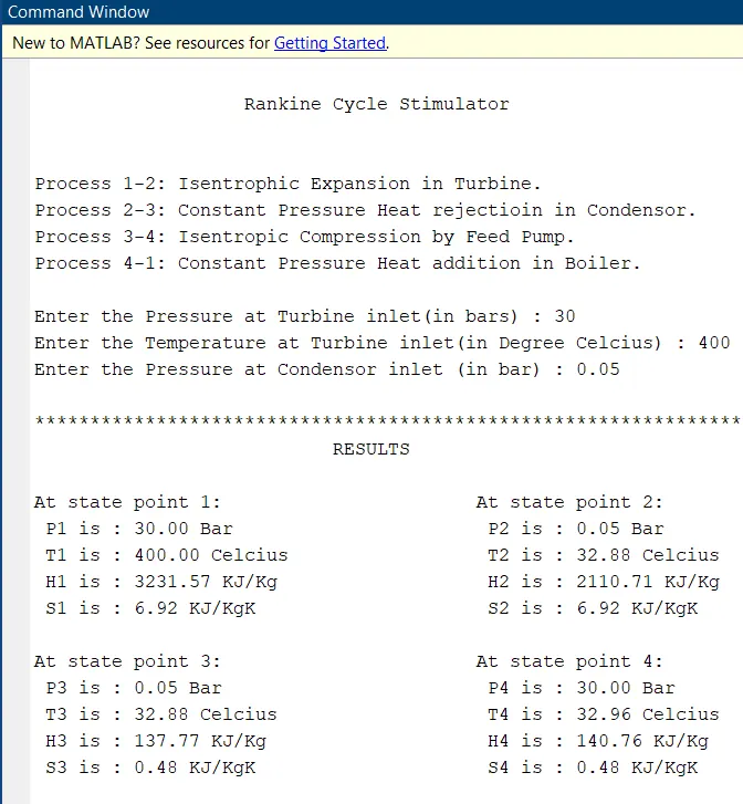
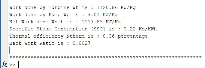
Commamd window
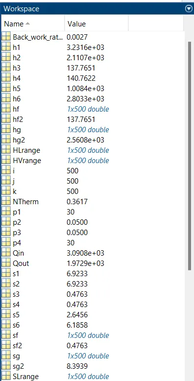
WorkSpace
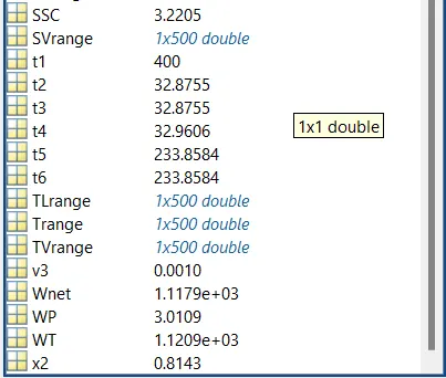
Plot for given input
Turbine Inlet temperature = 400° C
Turbine Inlet Pressure = 30 bars
Turbine Outlet Pressure = 0.05 bars = Condenser Inlet Pressure
1) T - S Diagram of Rankine cylce
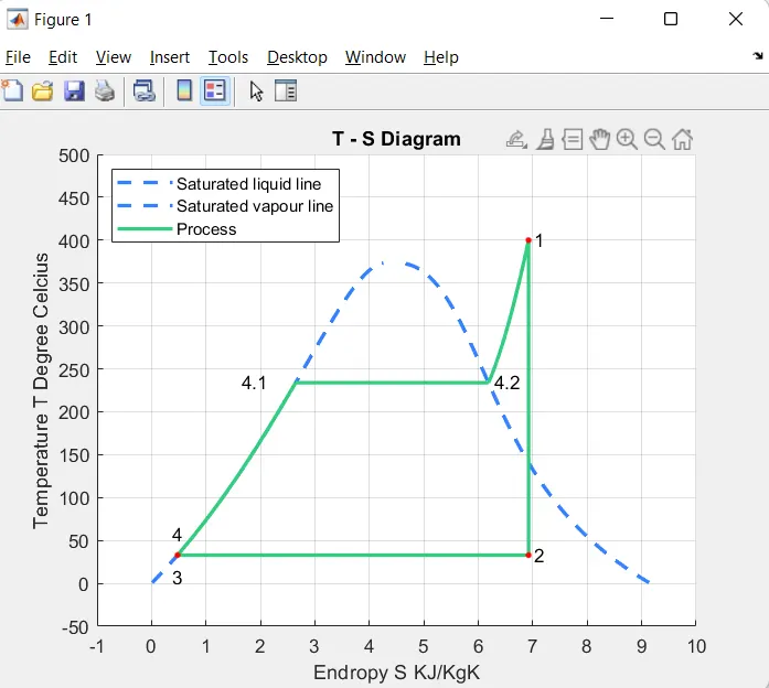
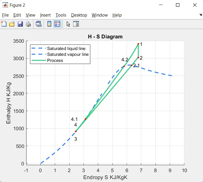
2) H - S Diagram of Rankine cycle
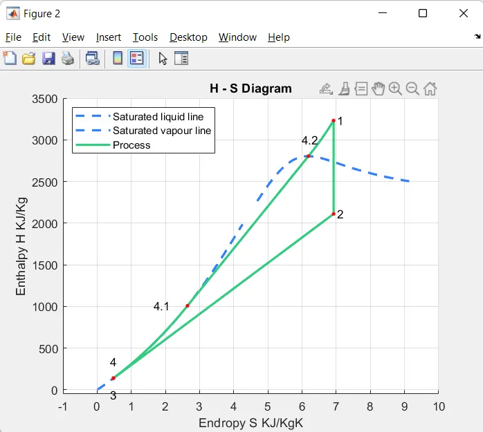
Plot during point 2 is at superheated region (steam entering condenser at superheated condition)
Turbine Inlet temperature = 500° C
Turbine Inlet Pressure = 70 bars
Turbine Outlet Pressure = 20 bars = Condenser Inlet Pressure
1) T - S Diagram of Rankine cylce
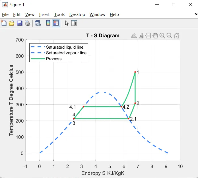
2) H - S Diagram of Rankine cycle
RESULT
- Simulated a Rankine cycle using matlab.
- Extracted Steam and water properties from XSteam data.
- Calculated all the state points of the cycle based on User inputs.
- Plotted the T vs s and H vs s plot for the given input.
- The Net work out put is obtained as 1117.85 KJ/Kg.
- The back work ratio was obtained as 0.0027.
Error
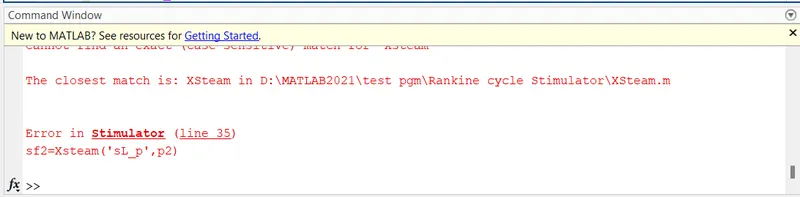
Miss spelled the library name
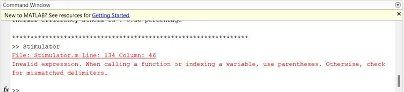
missing bracket
REFERENCES
https://en.wikipedia.org/wiki/Rankine_cycle