State of charge estimation
1.
The Battery Management System is a system that is used to predict the health and capacity of the charge in the battery. It is an electronic control circuit that monitors and regulates the charging and discharging of batteries. It is also used to determine the SOC and state of health of the battery. The main use of the BMS is the safety purpose to not reaching over currents and voltage and also the temperature.
The BMS not only monitors the values but also for the detection of battery type, voltages, temperature, capacity, state of charge, power consumption, remaining operating time, charging cycles, and some more characteristics.
The BMS model for simulation is downloaded from: https://in.mathworks.com/matlabcentral/fileexchange/72865-design-and-test-lithium-ion-battery-management-algorithms
Initially, the zip file is downloaded from the above link and then is loaded in SIMULINK. On opening the project from the plant folder the battery plant model is opened along with other files of the project. Further, the BMS system and the closed loop harness dashboard are opened. The BMS model consists of BMS ECU and a plant as shown below.
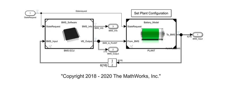
The controlling unit with various monitoring and control algorithms is connected to a block representing a battery pack. The battery pack may have a 6-cell series or a 16-module pack, each containing 6 cells in series. The below figure shows the content inside the BMS ECU.
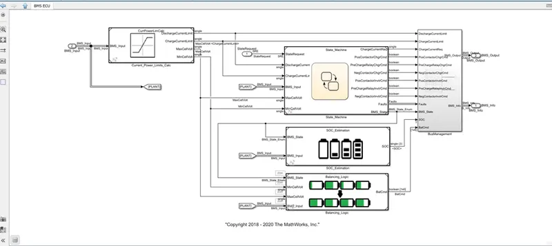
In this, as we can see that the main parameters were the current power limits calculator, state machine, SOC estimation, Balancing logic, bus management. From all the parameters the state machine is the main part which is the brain system or function of the BMS ECU. It takes the decision of controls the state of BMS, faults detections, its internal conditions etc. it takes the inputs as current limits, cell and pack voltages, cell temperatures, charger and inverter voltage outputs, pack current, state request, max and min cell voltages. The output from another side of the state machine are, the required charge current, BMS state, pre-charge relay charger and inverter command, positive contractor charger and inverter command, negative contractor charger and inverter command, and fault outputs. It is used to calculate the charge and discharge currents based on the given inputs.
In order to determine the SOC the SOC estimation block is used which consists of blocks as shown below.
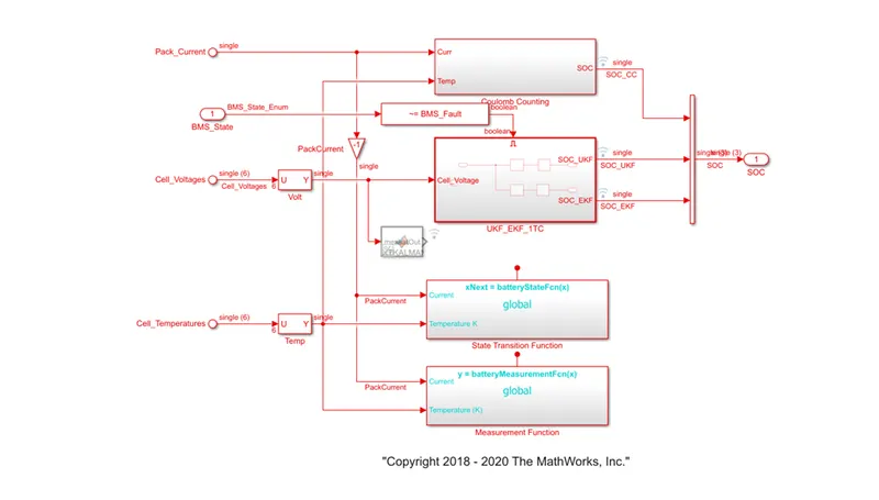
The pack current, the temperatures, the voltages and the BMS state are taken as inputs, the SOC is determined in 3 different ways they are by, column counting or by integrating pack current, Extended Kalman Filter (EKF) and Unscented Kalman Filter (UKF). We can see all the three SOC in the plots in the results section below.
The balancing logic subsystem again uses a state machine which is shown below,
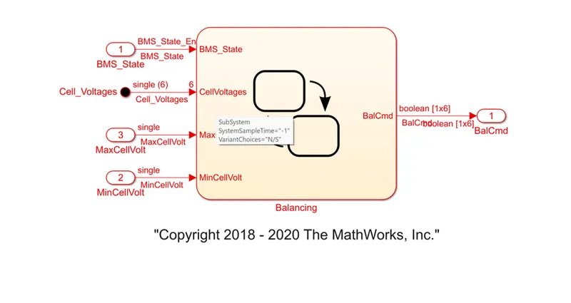
It takes the inputs as maximum vell voltage and minimum cell voltage, the cell voltage at that instant of time and the state of BMS and gives the output as a Boolean i.e., 0 or 1 indicating whether balancing is needed or not.
Coming to the plant subsystem, it takes the inputs from the BMS ECU and provides the feedback to the ECU the contents inside the subsystem is shown below.
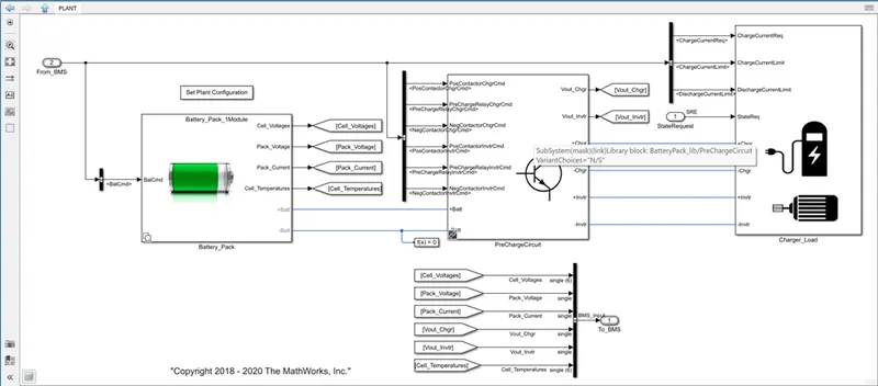
The subsystem consists of battery pack, pre charge circuit and a charger to charge or load to draw the current is attached. The battery pack has the inputs from the BMS and provides the outputs as cell voltage, cell temperature, pack voltage and pack current.
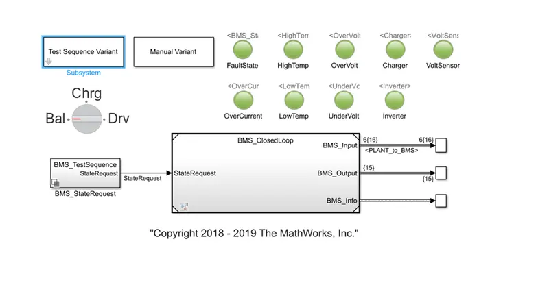
Now the test harness dashboard is opened in SIMULINK. Initially the model. The test hardness dashboard is the model which is used to test the BMS model outputs by changing the values of the given input to the BMS. By changing the values of the test conditions initially the model looks as shown below.
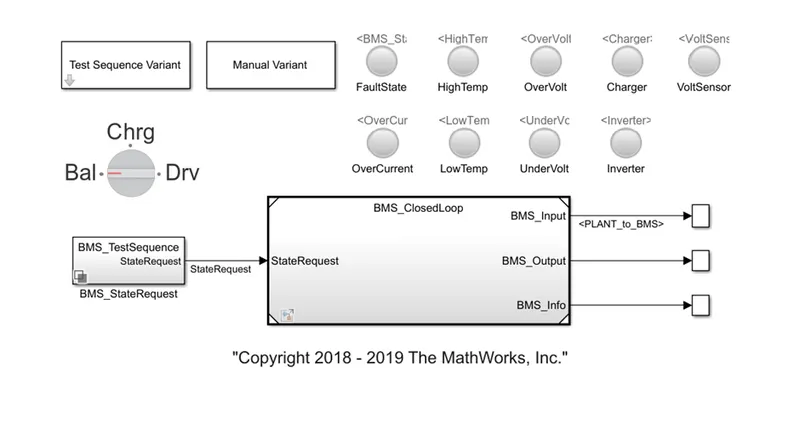
It has the lamps which are to detect the fault that occurred while simulation they glow green in normal conditions and red when faulty. The faults detected in the model are, fault state, over current, high temperature, low temperature, over voltage, under voltage, charger, inverter, volt sensor. There are three operating conditions in this model which the battery run in these 3 operations when it is on those are driving, charging and balancing which are shown in the rotary switch block.
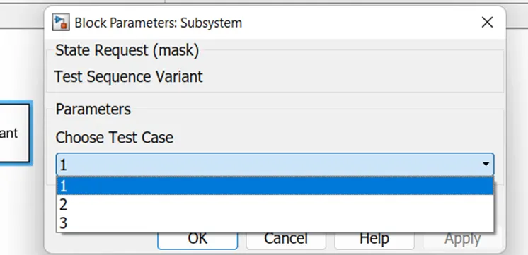
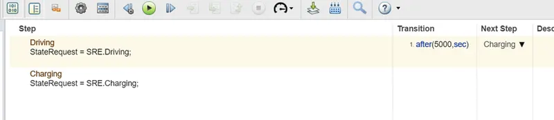
The model has three test conditions which can be configured from test sequence variant block as shown below. The test cases can be selected by selecting the required case from the dialogue box.
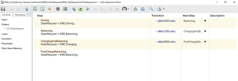
For test case 1,
The simulation is done for 20000 seconds, and for 3000 seconds it is in the driving state, and from 3001st second to the next 1000 seconds it is in the balancing state, further for the next 5000 seconds it is in the charging and balancing state and for the rest time it is in post charge balancing state.
On running the simulation at case 1 we can see the changes in the dashboard as shown below.
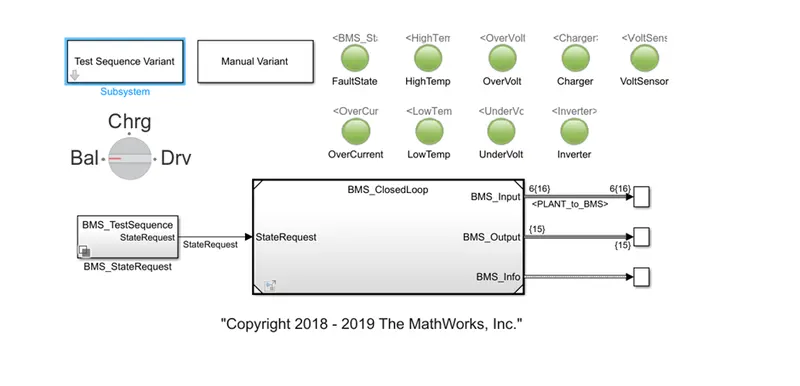
We can see that all the lamps are green in colour indicating that there is no fault occurring. The plots obtained at the end of the simulation for 1st case is shown below.
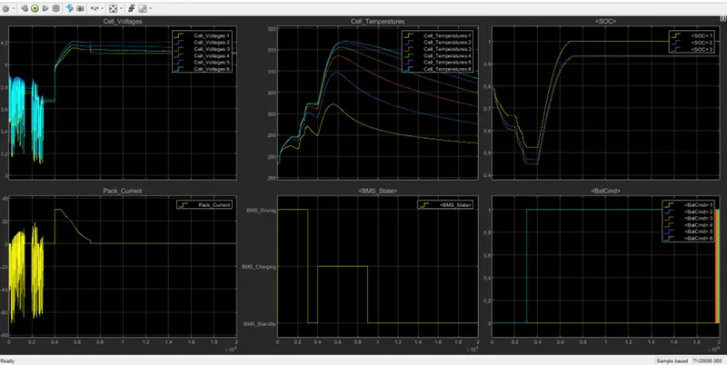
The first plot is for cell voltage while simulating the model the cell voltages are changing with the current flow. In the initial stage of simulation the, the voltages are slightly different because the model simulation was initialized with a slight associate of imbalance in the voltages are deflecting from 3.1V to 3.9V till the time period of 3000 seconds (Driving state). For the next 1000 seconds charging and balancing takes place we can see that the voltage reaches the peak value of 4.2 V which is attained at a faster rate due to constant current charging until the peak voltage once the peak voltage is attained at around 9000 seconds the cell balancing occurs as there is a decrease in voltage.
The next plot is for the temperature, we can see that temperature fluctuates normally during the driving state till 3000 seconds and then due to charging activities we can see the rise in temperature. The temperature rises drastically when the constant current is implemented. And further when the peak voltage is attained and when cell balancing starts we can see that the temperature drop down.
The next plot is of the SOC, we can see during the driving state the SOC keeps dropping down till 3000 seconds and once the charging occurs the SOC rises very fast. The plot represented in yellow is SOC determined by Columb counting method and the blue and red are for UKF and EKF respectively. We can see that the UKF and EKF are more accurate than the columb counting one as it does nor contain any sort of feedback. We can see that the SOC remains constant fro the further time period till the end of simulation i.e., 100% in case of the columb counting method, 93~94% in case of UKF and EKF.
The pack current plot, current fluctuates between +ve and -ve values during the driving state and once when the balancing starts the current value is 0. Further we can see that there is sudden rise in the value of current and then we can see the current is constant for some amount of time this is due to constant current charging. We can see that as the voltage is nearing to its peak value the current value starts to drop and the voltage is being constant as the current is dropping. Further after 9000 seconds only balancing occurs so the value of current becomes 0 till the end of simulation.
The next plot shows the state of BMS vs time, we can see as per our case till 3000 seconds the BMS is in driving state and after that period of time the BMS comes to stand by state i.e., balancing state for next 1000 seconds. Further as specified in our case charging state occurs for next 5000 seconds and after that again the balancing starts.
Now for test case 2,
Similar to case 1 the simulation is conducted for 20000 seconds. This test contains two states, driving till 5000 seconds and then the balancing state till end of simulation.
The dashboard after the simulation for test case 2 is shown below.
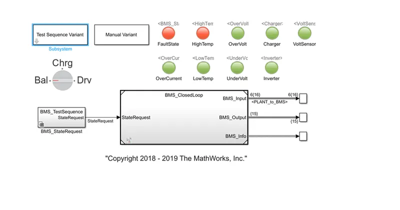
Similar to the case 1 the simulation was conducted for case 2 and we can see that two lamps are turned red. We can see that there is a fault state and high temperature. Rest of the lamps are green in colour indicating no errors.
The plots obtained after the simulation of test for case 2 is shown below.
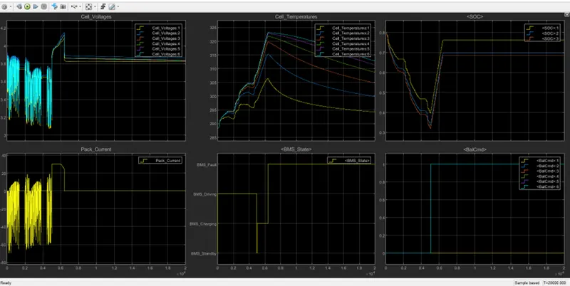
In the first plot, we can see that as specified in state the driving state till 5000 seconds, the voltage is fluctuating between 3.1V to 3.9V during this time duration. After 5000 seconds the charging occurs, where we can see the increase in voltage to the peak value. The voltage quicky rises up due to constant current supply the voltage then remains to be constant till the end of simulation.
In the temperature plot, the temperature fluctuates as the current and voltage fluctuates till 5000 seconds. Further more the temperature rises more than 320 and we can also see that the state is in fault state when the temperature crosses 320 value. This rise of temperature is because of usage of cells during first 5000 seconds and further its again charge by constant current as well.
Same as in test 1 case the SOC of the battery is reduces but in this case it been used even more as it is in driving state for more period of time. We can see that the SOC has dropped from 80% to almost 30%. However we can see that the UKF and EKF are more accurate and the SOC stops increases when the fault state occurs and remains constant for the rest of time.
The current also varies similarly as of the 1st test case while in driving state till 5000 seconds. Further as charge state occurs there is constant current occurring and as the voltage is nearer to its peak value the constant current change to constant voltage thereby seeing the drop in current value as voltage becomes constant. After the fault state the current remains at 0 till the end of simulation.
The remaining plots indicates the state of BMS with respect to time we can see that the BMS is in driving state till first 5000 seconds then in charging state and when temperature crosses the limit the fault state is attained.
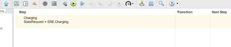
In the case 3, there is only one state happening i.e., only charging.
We can see that in our dashboard all the lamps glow green which indicates that there is nor error occurring.
The plots obtained after simulating for case 3 is shown below.
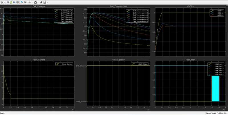
In the voltage plot we can see that the voltage rises for around 2000 seconds and then starts being constant for rest of the simulation time.
From the temperature plot we can see that the temperature is well withing limits and a slight amount of temperature is raised due to charging effect.
Since only charging is happening in this case we can see SOC raising only.
We can see that there is no constant current happening in any time period in this case as the voltage is already near its peak value so only constant voltage charging occurs and the current value is 0 when the SOC is at its maximum value till the end of simulation.
We can see that there is only one state occurring in the plot of BMS state that is charging.
2.
Coulomb Counting:
The Coulomb counting method measures the discharging current of a battery and integrates the discharging current over time in order to estimate SOC (State Of Charge). Or in other words, SoC Estimation by Coulomb Counting is based on the measurement of the current and integration of that current over time. The coulomb counting method is done to estimate the SOC, which is estimated from the discharging current and previously estimated SOC (State Of Charge) values, SOC is calculated by the following equation:
`SOC_(t) = SOC_(t-1) + (I(t))/(Q_n)delta(t)`
Where,
`SOC_(t)` = estimated State of Charge at time, t
`SOC_(t-1)` = previous State of Charge at time t-1
`I(t)` = charging or discharging current at time, t
`Q_n` = battery cell capacity
`delta(t)` = time step between t-1 and t
In this project, we can see the SOC estimation model in the BMS ECU,
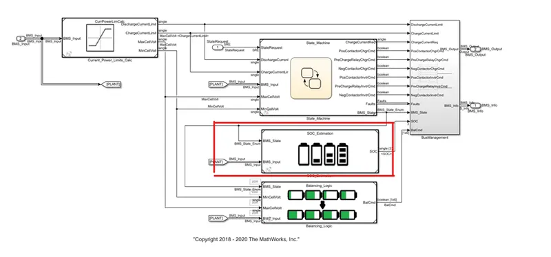
Further on opening that subsystem we see two different blocks for SOC estimation one by coulomb counting and the other by UKF and EKF.
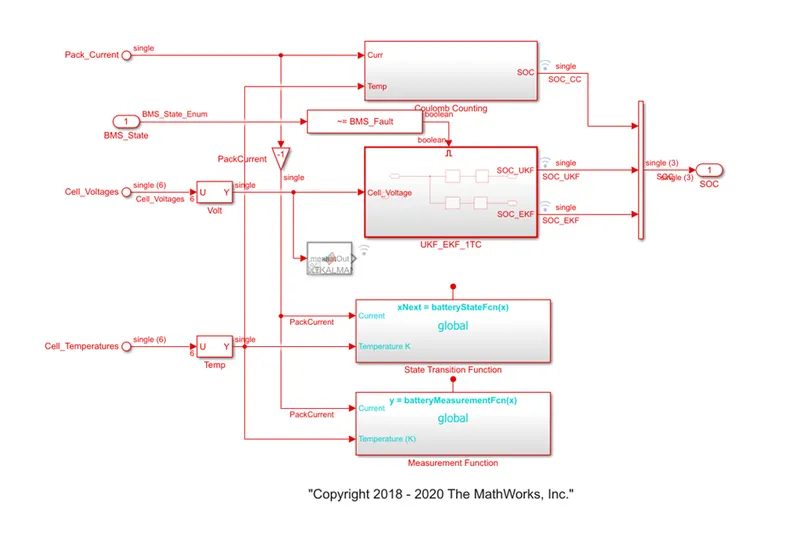
Inside the coulomb counting block it has various blocks such as, a gain (1/3600) block converting current to Ah, a 1-D lookup table for battery capacity for different temperature values, and a divide block to divide the current value by capacity at that temperature, and finally a discrete integrator block to integrate all the input signals.
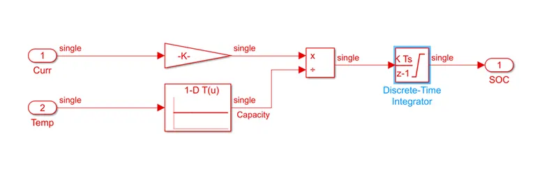
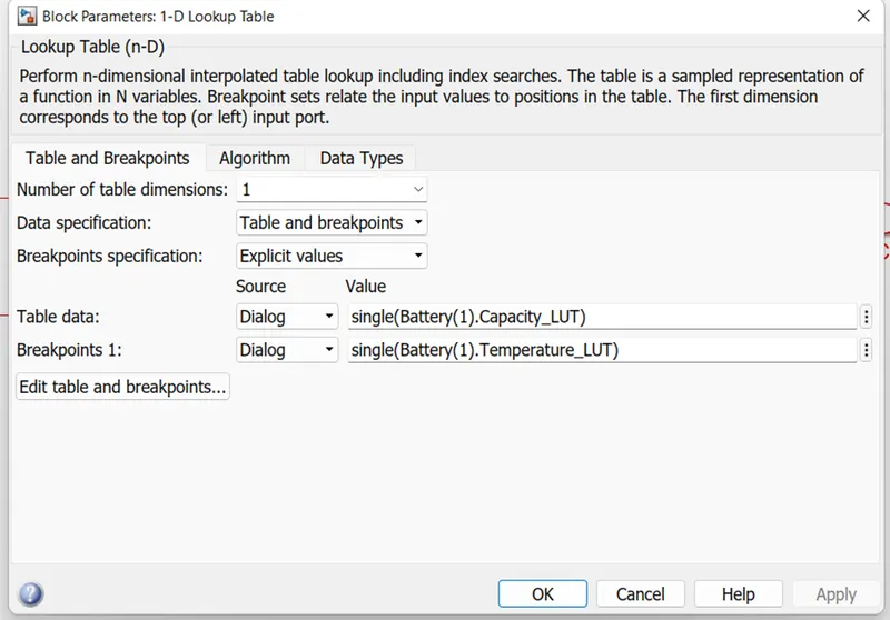
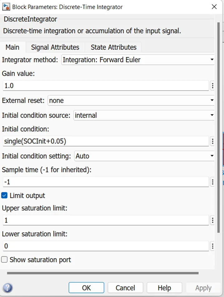
The blocks are implemented as the equation discussed in above section, current being converted to ampere-hour by the gain block. The capacity is determined with the value of temperature through the lookup table, further the current is divided by single cell capacity as shown in the equation above. The obtained value is for that instant of time hence it is integrated for overall value.
References:
https://www.batterydesign.net/soc-estimation-by-coulomb-counting/