Week 7 State of charge estimation

Aim: To estimate the state of charge.

Objective:

• To simulate the 3 test cases from the harness dashboard and to write a detailed report on the results.
• What is coulomb counting? Refer to the above model and explain how BMS implements coulomb counting for SOC estimation. 

Solution:

Case study 1:-Simulate the 3 test cases from the harness dashboard and write a detailed report on the results.

Downloading and opening closed-loop BMS harness dashboard model:

• Open the "Design and Test Li-ion Battery Management Algorithm" document in the file exchange.
• Extract the Zip file to a folder after downloading it. These files are contained in the folder, as shown below.

https://in.mathworks.com/matlabcentral/fileexchange/72865-design-and-test-lithium-ion-battery-management-algorithms

• Open Matlab and select Tests->System->BMS Closedloop Harness Dashboard model file to access the Simulink model file for the "Closed loop BMS harness dashboard."
• Give the pop-up dialogue box the option to open the project and the model to install all the model-related library files into the currently selected workspace and directories.

The BMS ClosedLoop Harness Dashboard model file is then opened as follows:

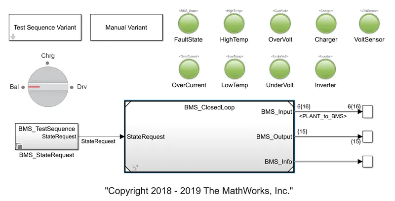
Model blocks:

(1) Dashboard

• Test Sequence Variant (Selector).
• Manual Modality (Selector).
• State request commands are provided by BMS Test Sequence (Subsystem).
• Lamps to signal voltage sensor operation, charging, high temperature, overvoltage, overcurrent, overcharging, inverter operation, low temperature, and Undervoltage. If there is any failure in these red indicators, we will be informed, and the green indicators show that everything is in fine shape.
• A rotating switch for manually changing variables while the simulation is ongoing.
  The outputs of the scope are the module's SOC, module current, individual cell voltages, individual cell temperatures, battery condition, and cell balancing states.

(2) BMS Closed loop

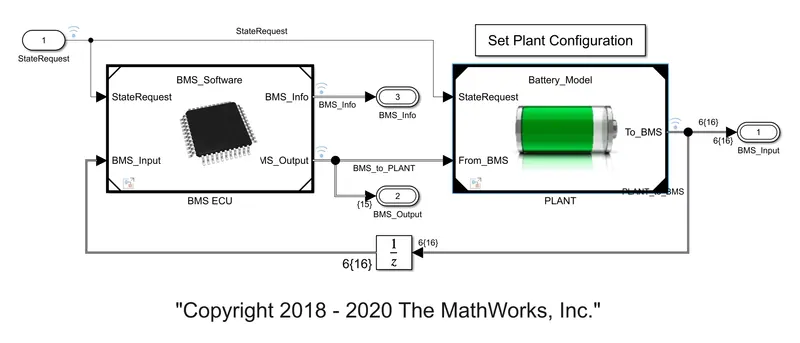
• BMS ECU and PLANT units are two of the subsystems in this primary block.
• The output of the plant is provided to the BMS ECU as input for the BMS input feedback loop.
• The BMS ECU unit receives the state request.
• The plant unit received the BMS Output commands as input marked "From BMS."
• The Plant unit receives the state request asap.
• BMS input, BMS Output, and BMs Info are the closed-loop model's final outputs.

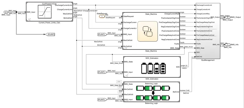
BMS ECU: The BMS ECU receives two types of input, including BMS Input, which is feedback from the Plant model, and the state request, which comes from the State Machine. This is producing output in the form of BMS Output and Info, which includes the logic for cell balancing, SOC estimation, and current power limit computation in state machines, as illustrated below.

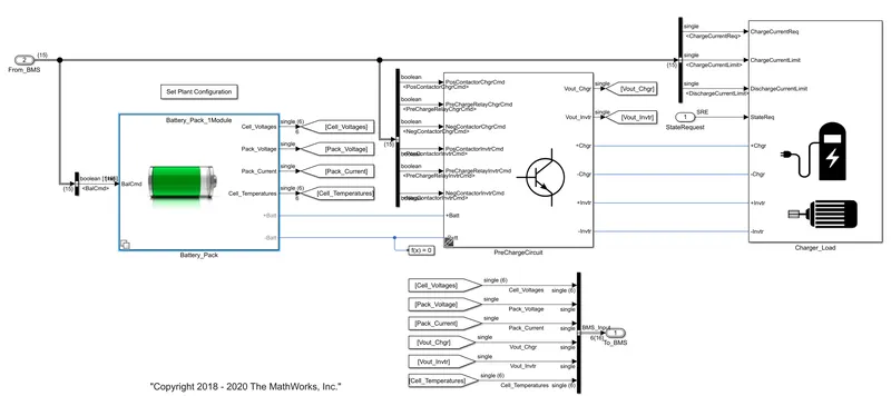
Plant: The system in question consists of a battery pack, a precharge circuit, and a charger and/or loads. There are two configurations in the battery pack: one module (6 cells) and sixteen modules (96 cells). Here, we've chosen just one module to make calculations simple and cut down on simulation time.

Discussions:

By choosing a test sequence variant and choosing each instance individually as a follow, we must test three scenarios for this model.

Test case 1:

In the test sequence variant dialogue box, choose 1 and click apply as displayed below.

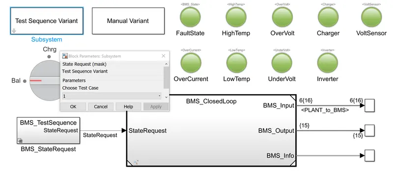
This selection consists of selection changes in masked BMS_State request subsystem as,

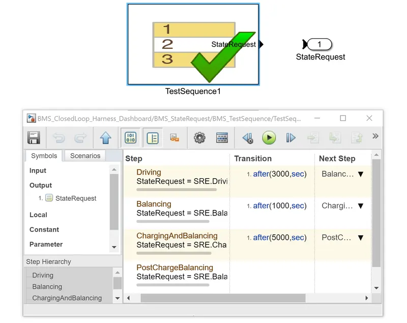
From the test sequence editor figure shown above, it was set as,

• First 3,000 seconds of driving.
• Balancing procedures start after 3000 seconds and last for the next 1000 seconds.
• The following 5000 seconds are spent on charging and balancing.
• Following that, until the completion of the simulation period, a series of post-charge balancing operations take place.

Results:

For the duration of the simulation, the lamp signals have been green, indicating that the sequences have been flawless.

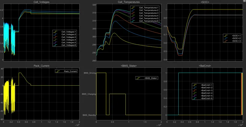
i) Driving (Discharging) mode (0-3000 sec):

• For the first 3000 sec, all cells are in driving mode, which causes them to discharge at a rate that fluctuates between 3.1 and 3.9 V. (min and max.).
• The temperature of the cell rises from 288 K to 302 K.
• SOC likewise declines for the EKF approach, going from 80% to 45%.

ii) Balancing mode (3000–4000 sec):

• Cell balancing takes place after 3000 sec and for 1000 sec, after which the modules enter standby mode and maintain a constant voltage of roughly 3.7V.
• As there is no current flowing through the cells when balancing, cell temperature slowly decreases.
• During this time, SOC, which is 45% for the EKF method, remains constant.

iii) Charging and Balancing (4000- 9000 sec):

• After 4000 sec, charging takes place, increasing the cell voltage from 3.7 to nearly 4.2 V in constant current mode with a current of about 30 A, and then constant voltage charging begins, reducing the current from 30 A to 2.6 A. Cells are charged and balanced for 9000 seconds.
• The temperature of the cell begins to rise exponentially up until the region of constant current falls as the current flow falls in the constant voltage mode.
• SOC for the EKF approach also rises in this mode from 45% to 94%.

iv) Post-charge balancing (9000–20000 sec):

• Following 9000 seconds, post-cell balancing begins in standby mode.
• In this state, the cell's temperature drops and it seeks to become closer to the surrounding temperature.
• SOC holds steady at 94%.

Test case 2:

Now select test case 2 and click apply in the test sequence variant dialog box as shown below,

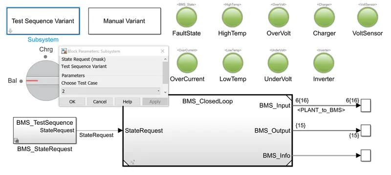
The case is altered to second as shown below,

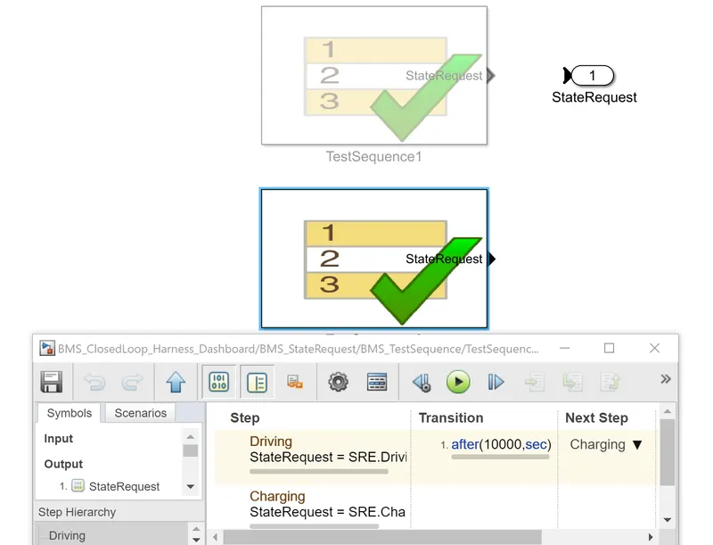
This test case consists of drive mode for 10000secs and after that charging occurs till the end of the simulation.

Results:

The model is fault-free because all states of the lamp's indicator are green.

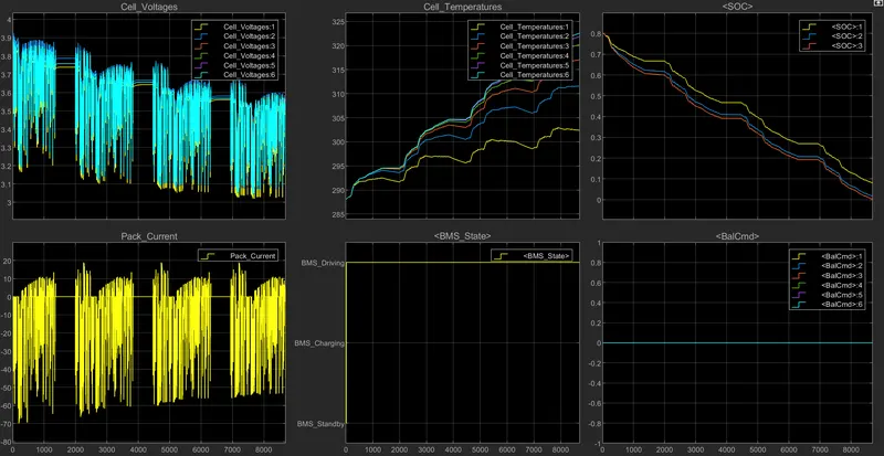
 i) Driving Mode (0-10000 sec): 

• The cell voltage varies from 3.9 V to 3.05 V, which is the cutoff voltage of the cell, and the full cell is drained for 8692 sec.
• The range of cell temperatures is 288 K to 322.5 K.
• In the driving mode, SOC decreases from 80% to 0% (cell is totally drained) in less than 8692 seconds.

Here, cell balancing is not done.

ii) Charging Mode (10000–20000 sec):

• Before entering this mode, the cell has already been depleted.

Test case 3:

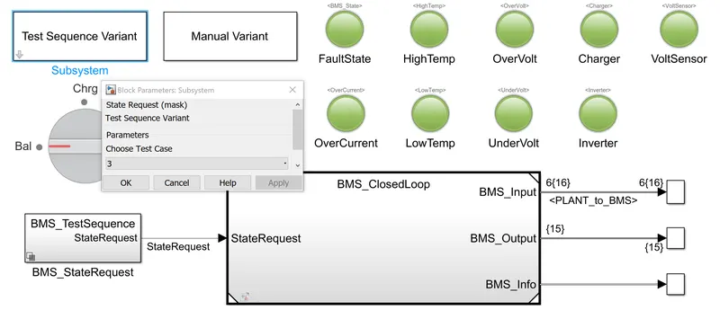
Now select test case 3 and click apply in the test sequence variant dialog box as shown below,

The test case is altered to third as shown below,

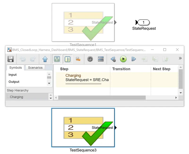
This test case consists of charging for the entire duration of time.

Results:

The model is fault-free because all states of the lamp's indicator are green.

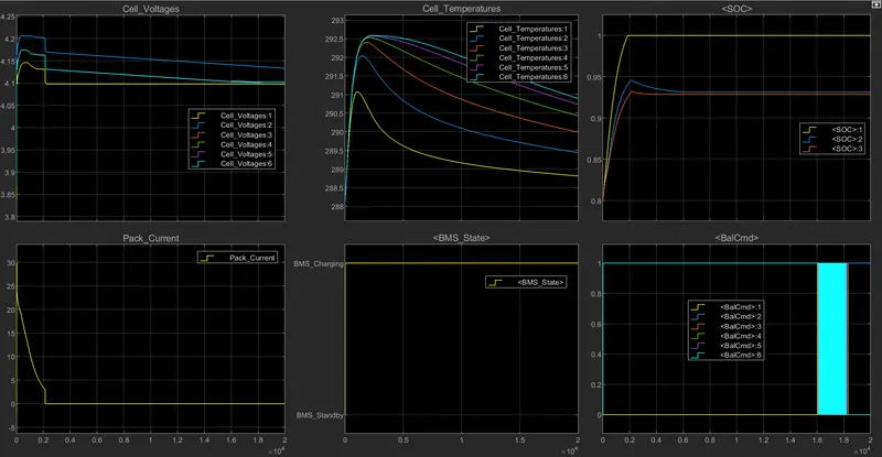
(i) Charging (0–2000 seconds):

• Cell voltages increased from their initial values and stabilized after 2000 seconds.
• The initial pack current ranges from 0 to 30 A, and after the constant voltage mode is enabled, the pack current starts to decline to 2.5 A and is fully charged within 2000 seconds.
• SOC started out at 80% and reached 100% after 2000 seconds of charging.
• Initial cell temperature increases are followed by a drop to ambient temperature once the battery is fully charged.

Case study 2:-What is coulomb counting? Refer to the above model and explain how BMS implements coulomb counting for SOC estimation. 

Coulomb Counting Method:-

The Coulomb counting method calculates SOC by measuring the battery's discharge current and integrating it over time. Using the discharging current, I(t), and previously calculated SOC values, SOC(t-1), the Coulomb counting method is used to estimate the SOC(t).

The following equation is used to determine SOC:

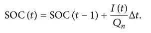
However, a number of variables, including temperature, battery history, discharge current, and cycle life, have an impact on the Coulomb counting method's accuracy.

Modified Coulomb Counting Method:-

A novel method termed the modified Coulomb counting method is put forth to enhance the Coulomb counting method. The corrected current is used in the modified Coulomb counting technique to increase estimation accuracy. The function of the discharging current is the rectified current. The corrected current and battery discharge current have a quadratic connection. The following formula is used to calculate adjusted current in practice using experimental data:

where k2, k1, and k0 are constant values obtained from the practice experimental data.

The following equation is used to determine SOC in the modified Coulomb counting method:

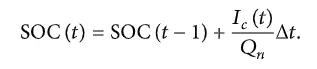
SOC estimation in Battery model:-

To observe the coulomb counting method we need to open the BMS_ClosedLoop>BMS ECU and then on SOC_ Estimation block

Here we see that there are three methods for calculation of SOC estimation and these are:-

i) Coulomb counting

ii) Unscented Kalman filter

iii) Extended Laman filter.

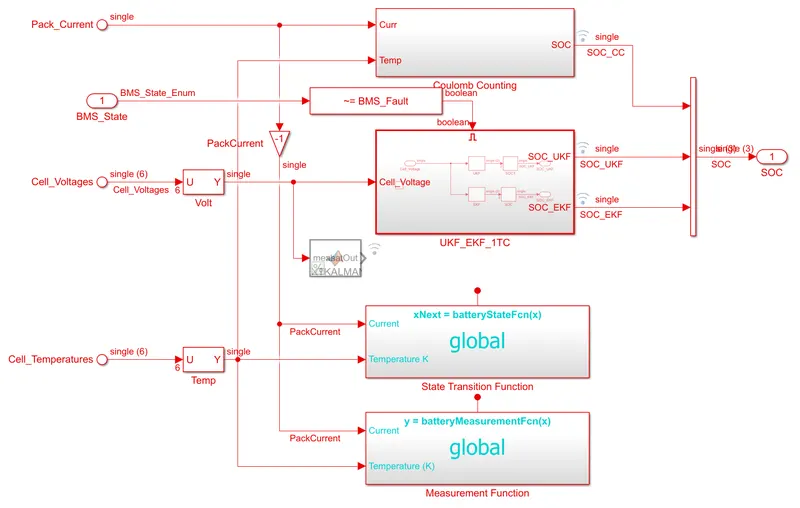
By opening the coulomb counting method we get to see the gain, 1-D look Up table, Product, and Discrete-Time Integrator block.

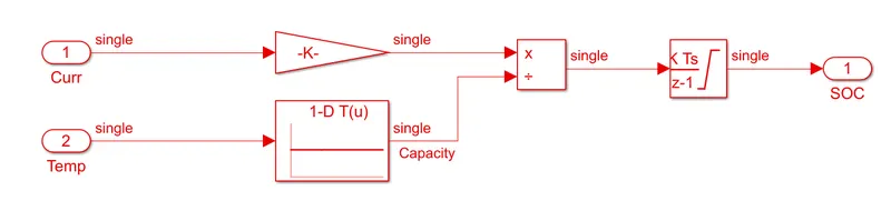
The discharge current from the battery is given to a gain having a value of 1/3600 to convert A to Ah.

That current is divided by the capacity due to temperature change and then integrated with the gain value of -1  wo=ith a sample time of -1 as a discrete type integrator is used here. The saturation limits are given which are 1 to 0. So that we get the SOC value from 0 to 1 multiplied by 100 to get the percentage of SOC.

Compared to the other two approaches, the Coulomb Counting method is simpler and takes less calculation.

The battery is used as a source of input for temperature and current. The gain block receives the current signal, while the capacity receives the temperature because it changes with temperature. These inputs are provided for integration, which will integrate the present relative to time. Another block receives this output, divides it by its capacity, and then estimates the SOC.