Project - Speed Control of a Direct Current (DC) motor

Aim: To develop a Simulink model for the DC motor using the Proportional, Integral, and Derivative (PID) control to design, develop and test a controller to maintain a desired speed for the motor.

Objective:

• Mathematical modeling from the first principles
• Modeling an Electrical Engineering system
• Simulink based modeling
• Control law design and test
• Stability of a dynamic system

Solution:

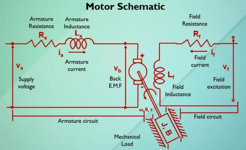
Mathematical modeling from the first principles:

• Using Kirchoff's voltage law

The algebraic sum of all voltage around any closed loop in a circuit is equal to zero.

Vs=Ra*ia+La(dia/dt)+Vb

• Back EMF, angular velocity & torque are related

Vb=Km(dθ/dt)

T=Kt*ia

Here, km and kt are the back emf and torque constants respectively

Angular velocity,ω=θdot

• The open loop transfer function for the motor with the speed (w) and supply voltage (vs) can be derived as

w(s)/Vs(s)=Kt/((J*La*S^2)+(J*Ra+B*La)S+(B*Ra+Kt*Km))

where,

Vs = Supply Voltage

Ra = Armature Resistance

ia = Armature Current

La = Armature Inductance

Vb = Back EMF

Modeling an Electrical Engineering system

• Parameters

(Jm) Moment of inertia of the rotor 0.01 kg.m^2

(Bm) Motor viscous friction constant 0.1 N.m.s

(Kf) Electromotive force constant 0.01 V/rad/sec

(Km) Motor torque constant 0.01 N.m/Amp

(Ra) Electric resistance 1 Ohm

(La) Electric inductance 0.5 H

• Control Design Objectives

Settling time < 2s

Overshoot < 5%

Steady-state error < 1%

• State Space Model

A = [-Bm/Jm km/Jm; -kf/La -Ra/La];

B = [0; 1/La];

Simulink based Modeling

PID Design for Speed control of DC motor:

%This file contains the design parameters to make a DC motor

%DC motor Parameters

Jm = 0.01; %Moment of Inertia of Rotor (Kgm^2)

Bm = 0.10; %Motor viscous friction constant (Nms)

kf = 0.01; %Back EMF constant (V/rad/s)

km = 0.01; %Motor Torque constant (Nm/Ampere)

Ra = 1.00; %Armature Resistance (ohm)

La = 0.50; %Armature Inductance (H)

%PD design

A = [-Bm/Jm km/Jm; -kf/La -Ra/La];

B = [0; 1/La];

%pole placement design

f = 1;

wn = 2*pi*f;

zeta = 0.5;

p1 = -zeta*wn + wn*sqrt(zeta^2-1);

p2 = -zeta*wn - wn*sqrt(zeta^2-1);

P = [p1;p2];

K = place(A,B,P);

Kp = K(1);

Kd = K(2);

Kp = 20;

Kd = -0.9;

Ki = 4;

Control Law Design and Test

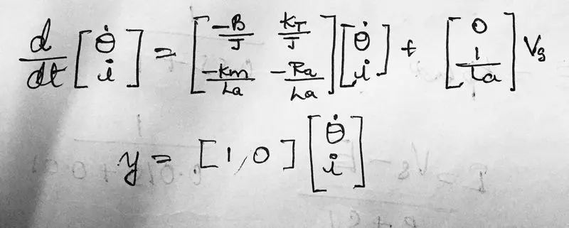
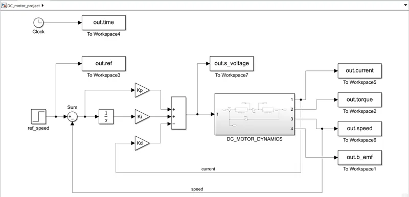
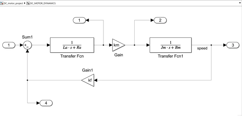
Design a PID controller to regulate the speed of the DC Motor.

• Consider the mathematical model of a DC motor.
• Select the P, I, and D gains such that the control design objectives for settling time, overshoot, and steady-state error are met.

• Simulation time(s)
• Start time: 0.0
• Stop time: 10.0
• Solver Selection
• Type: Fixed step
• Solver: ode4(Runge kutta)

• The reference signal is a Step Input signal
  • Step time:5s
  • Initial value:0
  • Final value:5

Kp and Kd value after pole placement method:

Kp = 20;

Kd = -0.9;

By tracking accurate ki manually from a value of 0 to 5, it is observed at Ki=4 desired output is obtained as required.

Stability of a Dynamic System

%ploting graphs of motor speed, supply voltage, current, torque, back emf

subplot(321);plot(out.time,out.s_voltage,'m--');grid;

subplot(322);plot(out.time,out.current,'m--');grid;

subplot(323);plot(out.time,out.torque,'m--');grid;

subplot(324);plot(out.time,out.b_emf,'m--');grid;

subplot(325);plot(out.time,out.ref,'b-');hold;grid;

subplot(325);plot(out.time,out.speed,'r-');grid;

subplot(325);xlabel('time');title('Speed(rad/s)');legend('Reference input speed','Motor output speed');

subplot(323);xlabel('time');title('Torque(Nm)');

subplot(322);xlabel('time');title('Current(A)');

subplot(321);xlabel('time');title('Supply Voltage(V)');

subplot(324);xlabel('time');title('Back EMF(V)');

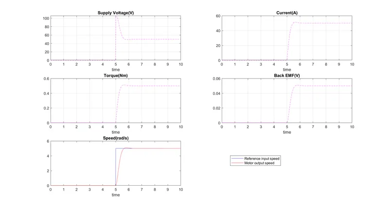
• The above plot shows the Speed signal with respect to the reference signal.
• The Blue signal is the reference signal from the step signal input.
• The red signal is obtained from the above circuit when feedback control gains Kd, Kp, Ki are applied.
• Here Kp=20.00 and Kd=-0.90 are found using the place command.
• By tracking accurate ki manually, the best signal is plotted in the above plot/graph at Ki=4.00.

Conclusion:

• Overshoot can be observed at less than 5%.
• Rise time can vary by controlling the Ki value.
• The settling time is less than 2s.
• Steady-state error is less than 1%.
• Equilibrium conditions are when it obtains a straight constant signal.