Challenge

Project 1

VVaishak Poojary10 Nov 2022

Aim: To develop a forward energy-based fuel consumption model of a conventional vehicle.

Objective:

Build a Simulink model using blocks and complete the vehicle model.
Writing scripts in MATLAB to load all the variables required for running the Simulink model.
Tabulate the fuel economy numbers (kmpl) for UDDS and HWFET cycles.
Plot the time trace for the engine, transmission input, transmission output, and wheel speed on one plot.
Plot engine torque, engine power, fuel rate, and fuel consumption using subplots.
Plot accelerator and brake pedal, gear command, vehicle desired and actual speed, and vehicle distance using subplots.
Plot the engine operating points on the engine fuel map.
Generate the plots for both drive cycles.
Study of Conventional vehicle Simulink model and creates graphs.

Solution:

Conventional Model: Conventional vehicles used are internal combustion engines fuelled by foil fuels to produce power for the wheels. Whereas Electrical vehicles use electric energy more than conventional internal combustion engines.

Conventional powertrain efficiency: The engine generates power by converting chemical energy stored into mechanical energy through the process of combustion. This process of energy conversion also has efficiency and the energy input is in the form of fuel consumption.

`dotmf = (Pe )/ (ηe * ηt * Q L H V)`

Where,

mf = mass flow rate in [kg]

pe = Power of engine

pt = power of transmission

nt = efficiency of transmission

ne = efficiency of the engine

QLHV = it is the calorific value/ lower heating value of the fuel.

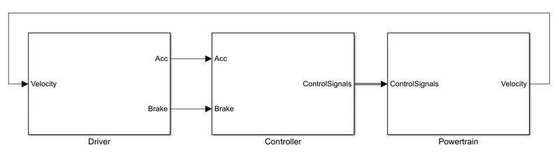
In this model, We use Forward Model: It is also known as dynamic simulation. Dynamic models are used for detailed simulations. In this model force/torque/power is the input and the vehicle state variable velocity and acceleration are the outputs. The models and simulations are more realistic due to physical casualty hence appropriate for control development. There is a feedback loop to meet the desired vehicle state. It is mainly used to simulate a vehicle on a driving cycle to analyze the dynamic behavior of the system helps significantly in control development.

Reference: https://www.researchgate.net/figure/Forward-facing-dynamic-vehicle-model_fig1_256202589

MATLAB scripts:

%% Skill-Lync -> Hybrid Drives Development

% Project 1 - Conventional Vehicle Model

% By - Vaishak

% Description:

%% Initialization File

% Initialization file for loading the variables for the Conventional vehicle simulation model

%% Vehicle Parameters

M = 1500; % Vehicle weight [kg]

Cr = 0.015; % Rolling resistance coefficient

Rw = 0.35; % Rolling radius [m]

Cd = 0.33; % Drag coefficient

Af = 2; % Frontal area [m2]

rhoa = 1.225; % Air density [kg/m3]

Vwind = 0; % Wind velocity [kmph]

g = 9.81; % Gravitational acceleration [m/s2]

theta = 0; % Slope [deg]

myu_road_tire = 1; % Coefficient of friction between tire-road interface

%% Powertrain Parameters

FDR = 3.73; % Final Drive Ratio / Diff Ratio

DiffEff = 0.99; % Differential efficiency (assumed independent of operating conditions)

NumGear = 4; % Number of gears in the transmission

TransGear = 1:NumGear; % Transmission Gears

TransRatio = [3.06, 1.62, 1, 0.7]; % Corresponding Transmission ratios

TransEff = 0.90; % Transmission efficiency (assumed independent of operating conditions)

TC_SR = [0, .5, .6, .7, .8, .87, .92, .94, .96, .97, 1]; % Torque Converter Speed Ratio (Matlab default) -> TurbSpd/PumpSpd

TC_TR = [2.232, 1.5462, 1.4058, 1.2746, 1.1528, 1.0732, 1.0192, 1, 1, 1, 1]; % Torque Converter Torque Ratio (Matlab default) -> TurbTrq/PumpTrq

TC_Cf = 1e-4 * [.72558, .66322, .63463, .59042, .51331, .4144, .29287, .22444, .12186, .04386, 0]; % Torque Converter Capacity Factor (Matlab default) -> PumpTrq/PumpSpd^2 [Nm/rpm^2]

load Vehicle_Data/Engine_data_1_9L_Saturn_95kW

load Vehicle_Data/Trans_Shift_map

%% Driver Parameters

Kp = 10; % P gain for driver PI model

Ki = 1; % I gain for driver PI model

Drive_Cycle_Select = 1; % Drive cycle selection

% Drive cycle values in m/s

if Drive_Cycle_Select == 1

load DriveCycles/UDDS;

elseif Drive_Cycle_Select == 2

load DriveCycles/HWFET;

elseif Drive_Cycle_Select == 3

load DriveCycles/FTP;

elseif Drive_Cycle_Select == 4

load DriveCycles/US06;

elseif Drive_Cycle_Select == 5

load DriveCycles/NEDC;

elseif Drive_Cycle_Select == 6

load DriveCycles/WLTP;

end

time_end = cyc_time(end);

vel_end = cyc_vel(end);

Simulink model of conventional vehicle:

In this project, a typical midsize car with a 1.9L engine and a 4-speed automatic transmission is considered. Data is taken from the ADVISOR database developed by NREL, USA. The transmission shift map and controller are taken from Matlab/Simulink example database.

Driver Model:

It is modeled using a ‘Driver’ block, which is a basic PI controller that generates accelerator and brake pedal outputs to match the desired and actual vehicle speeds. In this we use drive cycles and based on these results of fuel consumption and emissions the vehicle gets certified and it also forms a basis for uniform assessment. It is based on time, and velocity then it is all integrated and creates an output acceleration pedal and a brake pedal.

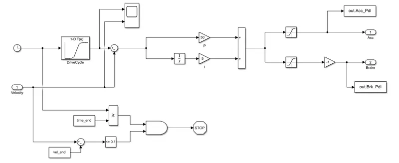
Control Model:

The ‘Controller’ block is the brains of the vehicle, representing the electronic control units. It is based on the driver inputs, it generates desired engine torque, desired transmission gear, and desired brake torque. These inputs are fed to the ‘Powertrain’ block which represents the drivetrain of the vehicle.

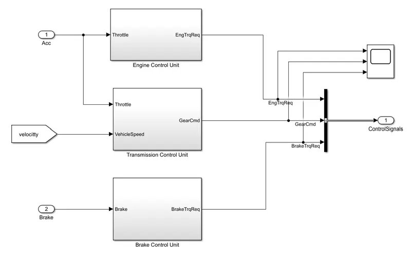
Engine Control Unit: In this control model We use an engine control unit that gives input Engine speed by creating a look-up table. in that table, we give input Maximum torque and map speed then also create a 2nd lookup table that gives input ct torque and map speed then it substracts and multiplied. the engine speed also gives to ideal control speed to integrate from this we meet the output of the engine's required torque.
Transmission Control Unit: In this unit, we create a steady flow variable state for controlling of gears of the vehicle in ascending and descending order with respect to time, speed, and distance. and give input to this steady state is vehicle speed in m/s to mph.
Brake Control Unit: In this calculate brake torque and then all three control signals output is given to the powertrain.

Powertrain:

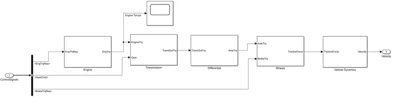
The powertrain encompasses every component that converts the engine's power into movement. This includes the engine, transmission, driveshaft, differentials, axles; basically anything from the engine through to the rotating wheels.

Engine

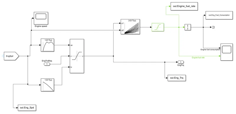
In this model, we used the map-based model to model the fuel consumption of the engine. It is based on maximum Torque and minimum torque from the controller. and then it saturated torque and gives output then saturated torque and the speed map gives fuel consumption takes the speed and torque then the output goes into saturated then it's integrated.

Transmission

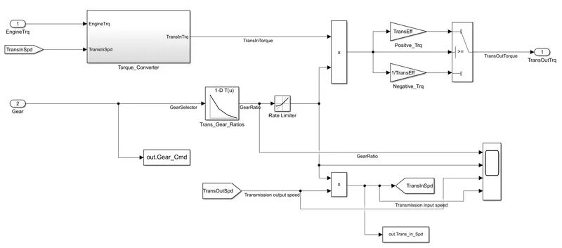
In these models, we take engine torque, and gear selector from the controller for transmission of gear ratio. The ratio is multiplied by the transmission input torque and then the transmission efficiency positive torque and negative torque give the transmission input speed. In this case, the torque converter connects the engine to the transmission it is part of the transmission. In it basically, engine dynamics are decoupled.

Differential

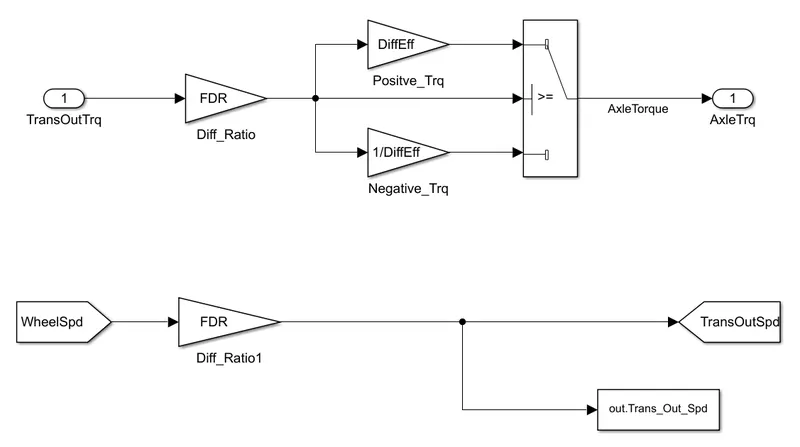
In this taking input is the transmission output then it's going to the differential ratio multiplied by the output and input torque then meets axle torque. The axle torque is lower than the transmission torque and differential ratio.

Wheels

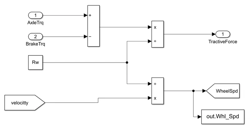
In this model, we take the axle torque from the differential and the brake torque from the controller. it is substracted and multiplied by the rolling radius and velocity then we meet the tractive force from the axle and brake torque. and the wheel speed is met using velocity.

Vehicle Dynamics

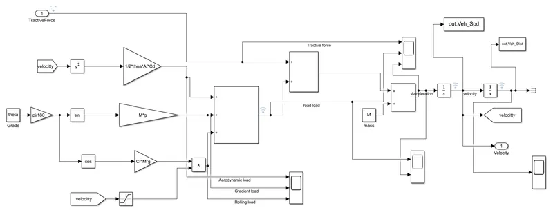
This takes tractive force and road load. It dictates vehicle speed based on tractive force and road load. The dynamic equation for calculating road load is

M_eq(dV_veh/dt) = [(η_t*λ_tot)/(R_w)] *T_m− [0.5*ρ*A*C_d*(V_veh+V_w_n_d) ^2+C_r*M*g*cos(θ)+M*g*sin(θ)]

where,

p = air density [kg/m^3]

A = Frontal area [m^2]

Cd = Drag Coefficient

Vveh = velocity of vehicle [m/s^2]

Vwind = velocity of wind [m/s^2]

Cr = rolling resistance coefficient

M = mass in [Kg]

g = gravity.

Then we calculate and integrate we meet acceleration of the vehicle and velocity of the vehicle which means vehicle distance and vehicle speed.

MATLAB scripts:

% The following file is to use with the Initialization file and Simulink

% results for post-processing of the data.

% The file is incomplete and has some examples of how the data is imported

% into a readable format, data analysis, and plotting examples.

% Based on the project task, use commands in a similar format as given

% below, to analyze the data and generate the required plots.

% You can change variable names if desired

%% Post-Processing File

% File for post-processing the Conventional vehicle simulation model data

%% Renaming variables

Time = out.tout;

Acc_Pdl = out.Acc_Pdl; % Accelerator pedal [%]

Brk_Pdl = out.Brk_Pdl; % Brake pedal [%]

Gear_Cmd = out.Gear_Cmd; % Transmission gear

Trans_In_Spd = out.Trans_In_Spd*30/pi; % Transmission input speed [rpm]

Trans_Out_Spd = out.Trans_Out_Spd*30/pi;% Transmission output speed [rpm]

Eng_Trq = out.Eng_Trq; % Engine brake torque [Nm]

Eng_Spd = out.Eng_Spd*30/pi; % Engine speed [rpm]

Eng_Fuel_Consump = out.Eng_Fuel_Consumption; % Engine fuel consumption [g]

Veh_Dist = out.Veh_Dist/1000; % Distance traveled by vehicle [km]

Veh_Spd = out.Veh_Spd*18/5; % Vehicle speed [kmph]

Wheel_Speed = out.Whl_Spd; % Wheel speed [kmph]

Eng_Fuel_Rate = out.Engine_fuel_rate; % Engine fuel rate [%]

%% Data Analysis

Eng_Pwr = (Eng_Spd.*pi.*Eng_Trq)./(30*1000); % Engine brake power [kW]

rho_petrol = 0.7197; % Density of petrol [kg/L]

kmpl = Veh_Dist(end)./(Eng_Fuel_Consump(end)/1000/rho_petrol); % Fuel economy [kmpl]

%% Plotting vehicle characteristics time trace

% for engine, transmission input, transmission output, and wheel speed

figure(1)

subplot(3,1,1)

hold on

grid on

plot(Time, Eng_Spd, 'linewidth', 1, 'Color', 'blue');

ylabel('Speed [rpm]')

xlim([0, Time(end)]);

legend('Engine Speed');

subplot(3,1,2)

hold on

grid on

plot(Time, Trans_In_Spd, 'linewidth', 1, 'Color', 'black');

plot(Time, Trans_Out_Spd, 'linewidth', 1, 'Color', 'red');

ylabel('Speed [rpm]')

xlim([0, Time(end)]);

ylim([0, 6000]);

legend('Trans Input','Trans Output');

subplot(3,1,3)

hold on

grid on

plot(Time, Wheel_Speed, 'linewidth', 1, 'Color', 'blue');

xlim([0, Time(end)]);

xlabel('Time [s]');

ylabel('Speed [rpm]');

legend('Wheel Speed');

%% Plotting engine torque, engine power, fuel rate, and fuel consumption

figure(2)

subplot(2,2,1)

plot(Time,Eng_Trq,'linewidth',1,'color','black')

xlabel('Time [s]')

ylabel('Torque [Nm]')

legend('Engine Torque')

grid on

subplot(2,2,2)

plot(Time,Eng_Pwr,'linewidth',1,'color','blue')

xlabel('Time [s]')

ylabel('Power [KW]')

legend('Engine Power')

grid on

subplot(2,2,3)

plot(Time,Eng_Fuel_Rate,'linewidth',1,'color','red')

xlabel('Time [s]')

ylabel('Fuel Rate [%]')

legend('Engine Fuel Rate')

grid on

subplot(2,2,4)

plot(Time,Eng_Fuel_Consump,'linewidth',1,'color','green')

xlabel('Time [s]')

ylabel('Fuel Consumption')

legend('Engine Fuel Consumption')

grid on

%% Plotting accelerator and brake pedal, gear command, vehicle desired and actual speed, vehicle distance

figure(3)

subplot(2,2,1)

hold on

grid on

plot(Time, Acc_Pdl, 'linewidth', 1, 'Color', 'black');

plot(Time, Brk_Pdl, 'linewidth', 1, 'Color', 'red');

ylabel('Pedal [%]')

xlim([0, Time(end)]);

legend('Accel','Brake');

subplot(2,2,2)

hold on

grid on

plot(Time, Veh_Spd, 'linewidth', 1, 'Color', 'blue');

ylabel('Speed [rpm]')

xlim([0, Time(end)]);

legend('Vehicle Speed');

subplot(2,2,3)

hold on

grid on

plot(Time, Gear_Cmd, 'linewidth', 1, 'Color', 'red');

xlim([0, Time(end)]);

xlabel('Time [s]');

ylabel('Gear');

legend('Gear Command');

subplot(2,2,4)

hold on

grid on

plot(Time, Veh_Dist, 'linewidth', 1, 'Color', 'green');

xlim([0, Time(end)]);

xlabel('Time [s]');

ylabel('Distance [km]');

legend('Vehicle Distance');

%% Plotting engine operating points on the engine fuel map

figure(4);

hold on

grid on

title('Engine Operating Points','fontsize',12);

p1=plot(Eng_map_spd*30/pi,Eng_max_trq,'linewidth',2,'color','r');

p2=line([Eng_map_spd(end)*30/pi Eng_map_spd(end)*30/pi],[0 Eng_max_trq(end)]);

set(p2,'linewidth',1,'linestyle','--','color','k');

p3=line([Eng_map_spd(1)*30/pi Eng_map_spd(1)*30/pi],[0 Eng_max_trq(1)]);

set(p3,'linewidth',1,'linestyle','--','color','k');

[c,h] = contour(Eng_map_spd'*30/pi,Eng_map_trq,Eng_fuel_map');

clabel(c,h);

xlabel('Engine Speed [rpm]');

ylabel('Engine Torque [Nm]');

title('Engine Fuel Consumption Map [g/s]');

%p4 = plot(Eng_Spd,Eng_Trq,'.','color','k');

legend([p1 p3],{'Max Curve','Operating Points'});

axis([Eng_map_spd(1)*30/pi Eng_map_spd(end)*30/pi 0 Eng_map_trq(end)]);

Results:

Fuel economy numbers:

As we see, the fuel economy is high in HWFET compared to UDDS, it is because, in urban driving, the vehicle encounters more traffic and it has to stop for fewer distances and it consumes more fuel at the start. In HWFET, the vehicle encounters no traffic and it moves without the use of too much braking, so it will have more fuel economy number.

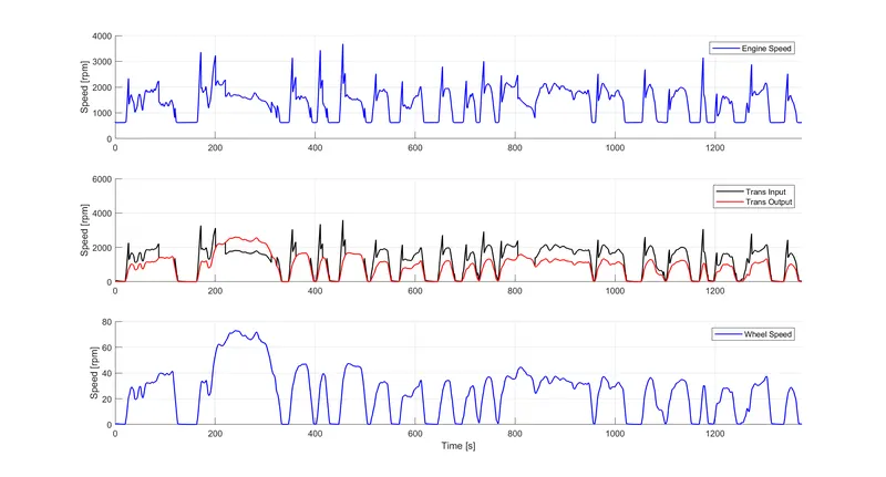
Plotting vehicle characteristics time trace for engine, transmission input, transmission output, and wheel speed:

UDDS drive cycle:

HWFET drive cycle:

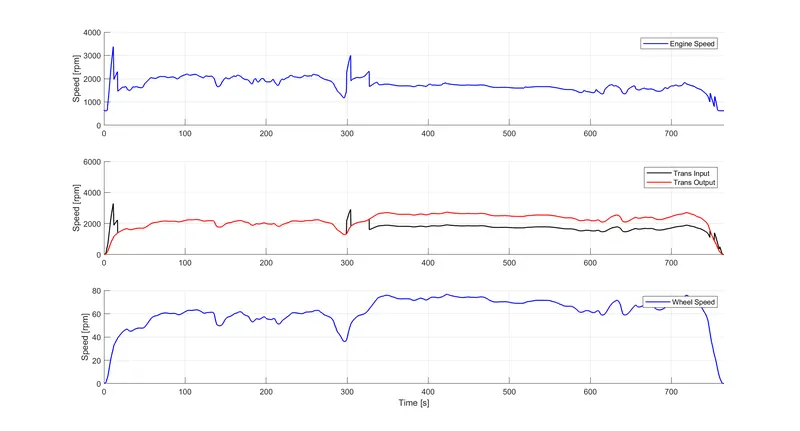
We can see that the graph has more fluctuations in UDDS compared to the HWFET cycle.
Braking is high in UDDS when compared to HWFET due to traffic Peak.

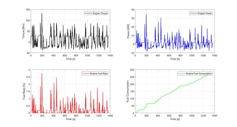
Plotting engine torque, engine power, fuel rate, and fuel consumption:

UDDS drive cycle:

HWFET drive cycle:

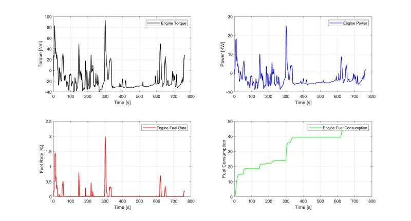
The vehicle consumed more power in the UDDS compared to the HWFET cycle because it has too many starts and stops compared to HWFET.
Engine torque is also high in UDDS because while starting from rest, the vehicle requires more torque to overcome static friction.
The fuel rate is high in HWFET because the vehicle will be in continuous movement, and it consumes more fuel.
The fuel economy will be high in HWFET compared to UDDS because there are many stops and starts in UDDS and more fuel is consumed when the vehicle is in an idle position.

Plotting accelerator and brake pedal, gear command, vehicle speed, and vehicle distance:

UDDS drive cycle:

HWFET drive cycle:

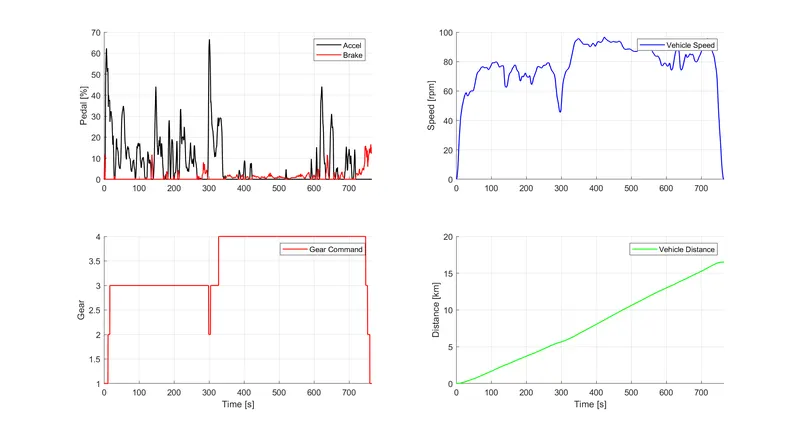
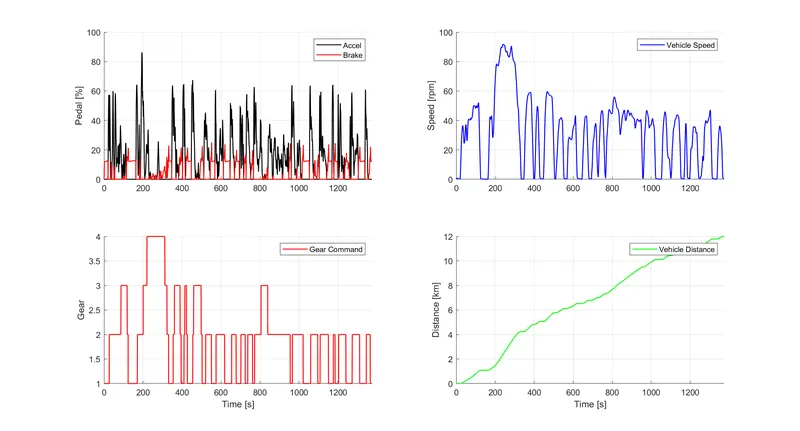
For UDDS, the accelerator and the brake pedal have more fluctuations because of frequent starts and stops. But in HWFET, the brake pedal fluctuations are almost near the zero line as there will be no frequent stops.
UDDS cycle mostly runs on 1st, and 2nd gears, and uses 3rd, and 4th gears very rarely as it does not achieve high speeds in that traffic. In the HWFET cycle, the vehicle mostly run on 3rd, and 4th gears as it will be moving at high speeds. It uses 1st, and 2nd gears very frequently when braking is required.
The vehicle speeds will be high in HWFET compared to UDDS. UDDS also has more fluctuations in speed due to frequent braking.
The distance traveled in the given time will be high in HWFET than in UDDS because of the traffic barrier in UDDS.

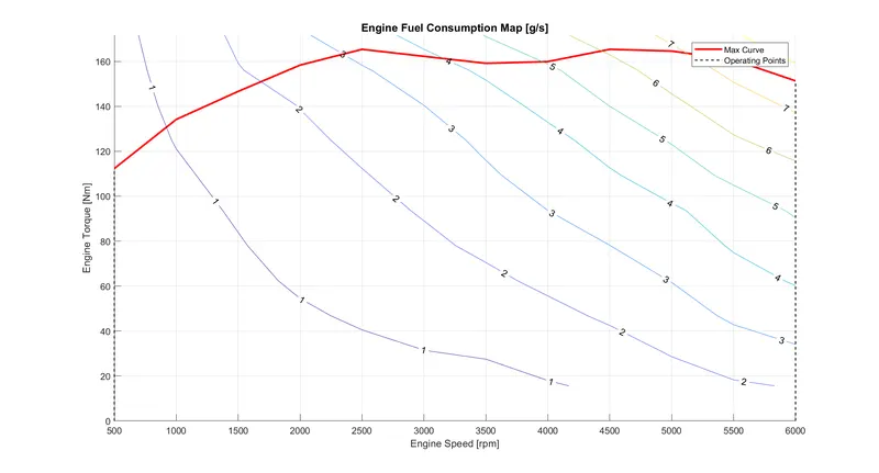
Plotting engine operating points on the engine fuel map:

UDDS drive cycle:

HWFET drive cycle:

By this, it is clear that as torque decreases speed increases.

Conclusion:

The fuel consumption rate is more in UDDS than in HWFET.
The UDDS drive cycle is best for asses of fuel consumption and Pollutant emissions of vehicles in a normalized way.
Distance traveled is more in HWEFT than in UDDS.
We can observe that in UDDS the efficiency of the engine & fuel consumption is lost in braking & gear changing the vehicle.

Project 1

Ship work like this
in your own course.

Talk to a career counsellor

Ship work like thisin your own course.

Talk to a career counsellor

Ship work like this
in your own course.