Week 7 State of charge estimation

Aim : To Simulate the 3 test cases from harness dashboard of Lithium ion battery management Algorithms (MATLAB Example project).

This example project can be used as a reference design to get started with designing Lithium Ion Battery Management System (BMS) with MATLAB and Simulink.

Project includes Simulink models for BMS Algorithms such as:

1. State of Charge estimation using Extended Kalman Filter, Unscented Kalman Filter
2. Passive Battery Cell Balancing
3. State Machine for Pre-charging and Contactor Management
4. Fault Management - Over/Under Voltage, Over Current, Over Temperature etc.
5. Charge and Discharge Current Limit Calculations

The Model:

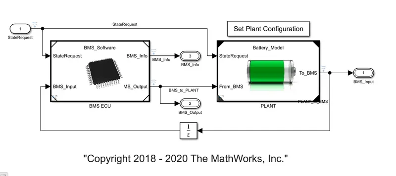
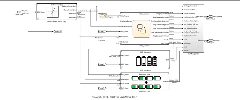
BMS ECU : represents the software and controls part of the model, showing how cell balancing is done, SOC is estimated, and response to different states(using stateflow)

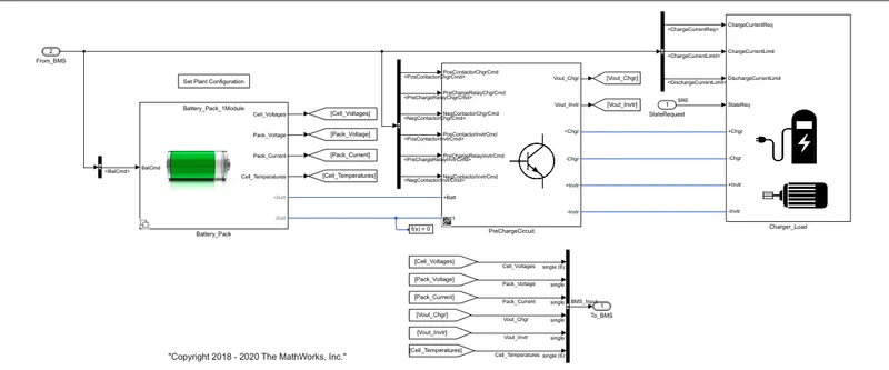
Plant: represents the hardware part of the model, with the battery pack, precharge circuit and charger.

Test Harness Dashboard: testing different scenarios and conditions.

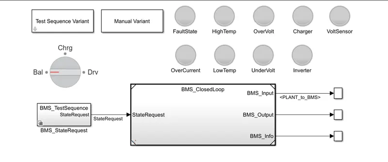
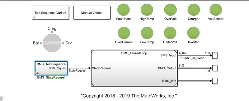
TEST CASE 1:

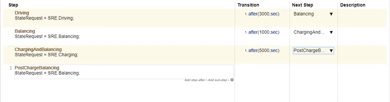
• Battery is in driving mode for first 3000 seconds.
• The next 1000 secs there is cell balancing as the BMS has come to a standby. This generally happens only when the vehicle has to stop for a long time.
• The next 5000 sec are for charging
• BMS continues to be in standby for the remaining 11000 seconds
• we got all indicators green so there's not any fault condition in battery.

Observations:

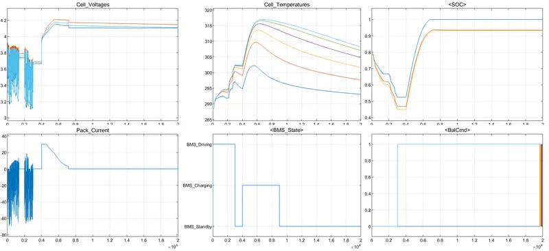
1. Fluctuations in cell voltages and pack current until 3000 sec indicates that the vehicle was in driving mode

2. Cell voltages start off differently which means there was SOC imbalancing from the beginning. However, they do start converging after 3000 sec as cell balancing begins, and by the end of 20,000 sec all cells stabilize around 4.l V

3. Between 4000 sec and 9000 sec there is constant current (CC) and constant voltage (CV) charging happening: from 4000-4600 sec it is CC and then the remaining is CV. During CC the SOC increases much more quickly, and then slows down during CV as a precaution mechanism to avoid charging past the voltage limit

4. There is a moderate difference in the temperatures of Cell 1 (297K) and Cell 6 (303K) when the vehicle comes to a stop at 3000 sec. This is because of the way the battery pack is assembled. Cell 1 is open to the atmosphere while Cell 6 is thermally insulated on oneside. The difference in their peak temperatures is 15 degrees C, and this happens during the initial charging stages. Even at the end of the simulation, when the BMS has been in stand by mode for > lOOOO sec the difference in temperature of cell 1 and cell 6 is still 15 degrees C. This really points to the importance of how vital it is to maintain a similar temperature throughout the wholepack, otherwise it will lead to difference between individual cells, such as their voltages, discharge capacities, cycle life or cell degradation, etc.

5. The SOC graph shows the estimation of SOC through different methods, with yellow corresponding to coulomb counting, blue for unscented Kalman Filter (UKF), and orange for Extended Kalman Filter (EKF). Both Kalman filter methods are evidently more accurate than coulomb counting due to their ability to account for voltage information (the difference between OCV and (sum of) voltage drops)

TEST CASE 2:

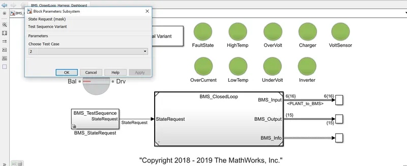
The first 10000 sec is driving mode then after that there is charging mode.

Observation:

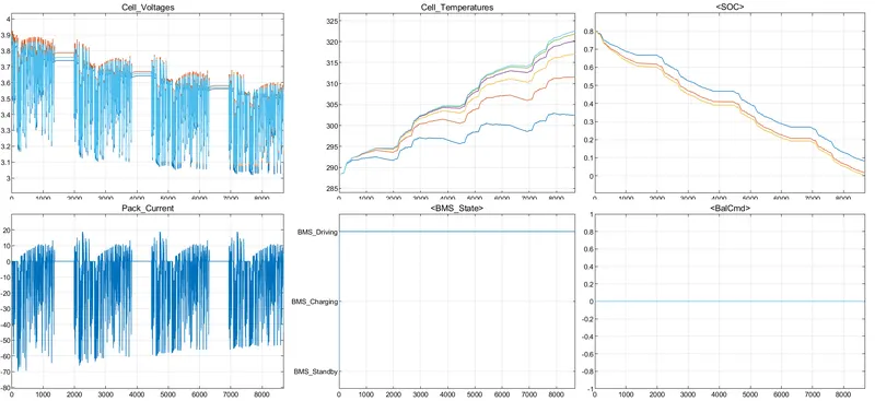
1. Cell voltage ranges from 3.9V - 3.05V aprrox. The pack current varies from -70A - 20A. Some negative current occurs because of drive cycle which works in regenerative mode
2. Both current and voltage works according to drive cycle and works as accelerated and deaccelerated mode. Entire capacity drained at 8693 sec
3. Cell 1 has least temp rise and cell 6 has high temperature rise
4. These cells temperature are increasing and decreasing as per driving and charging period.
5. SOC started from 80% and drained to 0% in driving mode only
6. Balancing of cell didnt performed in the entire cycle

TEST CASE 3:

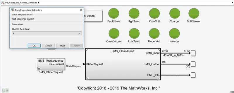
Only charging will be done in this case

Observations:

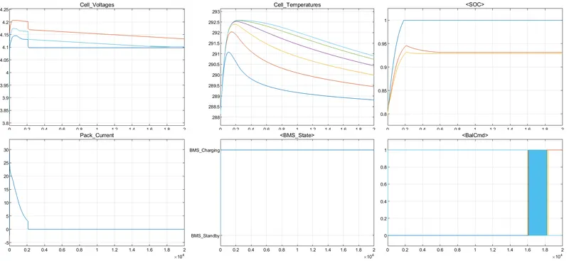
1. Since the battery is only in charging mode, the sudden influx of current from 0 to 30A is seen within the first 5 seconds (when zoomed in). Due to the surge of electrons into the cells, this also explains the drastic rise in temperature in all cells
2. Cell balancing is in process since the beginning
3. EKF has outperformed UKF by a little bit again, while Coulomb counting method for SOC approximation seems the most inaccurate one. we can say this because a SOC of 100% is highly unlikely, and with Coulomb counting it might be displaying 100% because it is only pre-programmed to do so at the end of CC CV charging. EKF shows a SOC of 93% while UKF displays 94.5%, which seem more realistic and accurate.

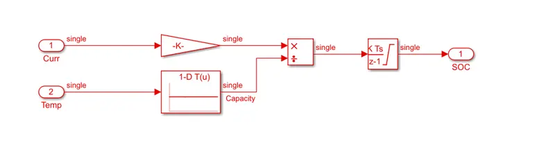
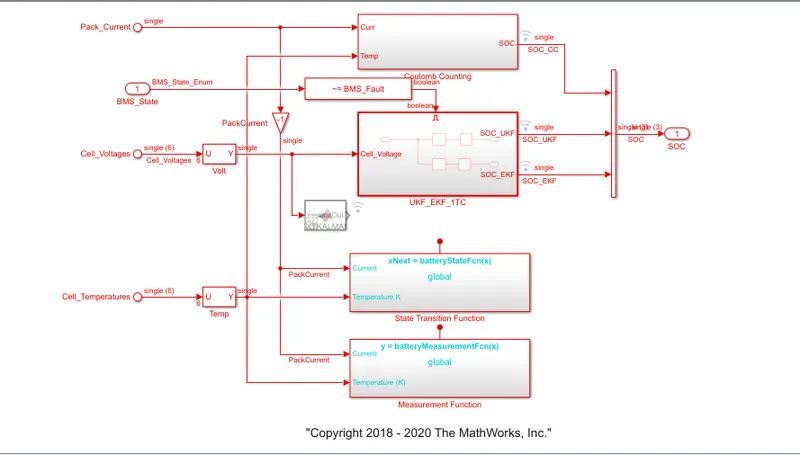
2.What is coulomb counting? Refer to the above model and explain how BMS implements coulomb counting for SOC estimation ?

Coulomb counting is a technique used to track the State of Charge of a battery pack. It works by integrating the active flowing current (measured in amps) over time to derive the total sum of energy entering or leaving the battery pack. This produces a capacity that is typically measured in Amp-hours.

The Coulomb counting method measures the discharging current of a battery and integrates the discharging current over time in order to estimate SOC . Coulomb counting method is done to estimate the SOC(t) , which is estimated from the discharging current,I(t) , and previously estimated SOC values,SOC(t-1) .

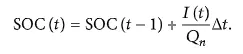
But there are several factors that affect the accuracy of Coulomb counting method including temperature, battery history, discharge current, and cycle life

Modified Coulomb Counting Method

To improve the Coulomb counting method, a new technique called modified Coulomb counting method is proposed. The modified Coulomb counting method uses the corrected current to improve the accuracy of estimation.

The corrected current is the function of discharging current. There is a quadratic relationship between the corrected current and discharging current of battery. By practice of experimental data, corrected current is calculated by the following form:

where ,k2,k1 and k0 are constant values obtained from the practice experimental data.

In modified Coulomb counting method, SOC is calculated by the following equation:

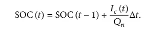
The experimental results show that the accuracy of the modified Coulomb counting method is superior to the conventional Coulomb counting method.