Week 4.1 - Genetic Algorithm

AIM: To study Genetic Algorithm to optimise the Stalagmite function and find global maxima in MATLAB.

OBJECTIVE:

• Write code in MATLAB to optimise the stalagmite function and find global maxima of function.
• Explain the concept of Genetic Algorithm and syntax for ga in MATLAB.
• Plot graphs for all studies and for F maximum vs no. of iterations.

Genetic Algorithm:

• A genetic algorithm (GA) is a method for solving both constrained and unconstrained optimization problems based on a natural selection process that mimics biological evolution. The algorithm repeatedly modifies a population of individual solutions.
• At each step, the genetic algorithm randomly selects individuals from the current population and uses them as parents to produce the children for the next generation. Over successive generations, the population "evolves" toward an optimal solution.
• We can apply the genetic algorithm to solve problems that are not well suited for standard optimization algorithms, including problems in which the objective function is discontinuous, nondifferentiable, stochastic, or highly nonlinear.
• The genetic algorithm uses three main types of rules at each step to create the next generation from the current population:
• Selection rules select the individuals, called parents, that contribute to the population at the next generation.
• Crossover rules combine two parents to form children for the next generation.
• Mutation rules apply random changes to individual parents to form children.

The genetic algorithm differs from a classical, derivative-based, optimization algorithm in two main ways, as summarized in the following table.

Syntax for GA:

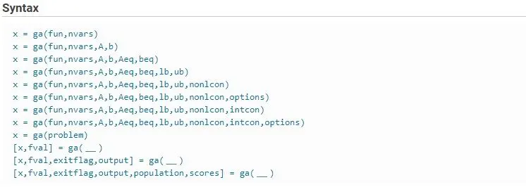
The ‘ga’ syntax in MATLAB is used to find the minimum of a function using a genetic algorithm. The syntax used for this study is shown below.

How the genetic algorithm works:

1. The algorithm begins by creating a random initial population.
2. The algorithm then creates a sequence of new populations. At each step, the algorithm uses the individuals in the current generation to create the next population. To create the new population, the algorithm performs the following steps:
   1. Scores each member of the current population by computing its fitness value. These values are called the raw fitness scores.
   2. Scales the raw fitness scores to convert them into a more usable range of values. These scaled values are called expectation values.
   3. Selects members, called parents, based on their expectation.
   4. Some of the individuals in the current population that have lower fitness are chosen as elite. These elite individuals are passed to the next population.
   5. Produces children from the parents. Children are produced either by making random changes to a single parent—mutation—or by combining the vector entries of a pair of parents—crossover.
   6. Replaces the current population with the children to form the next generation.
3. The algorithm stops when one of the stopping criteria is met.
4. The algorithm takes modified steps for linear and integer constraints.
5. The algorithm is further modified for nonlinear constraints.

Stalagmite Function:

A stalagmite is an upward growing mound of mineral deposits that have precipitated from water dripping onto the floor of a cave. Most stalagmites have rounded or flattened tips.

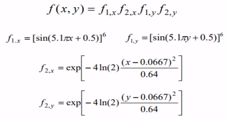
A stalagmite function generally refers to the function with which we are generating values over a stalagmite kind of surface for finding out the local and global maxima and minima of that particular given function.

In MATLAB we use this function for optimisation.

MATLAB PROGRAM:

1) Stalagmite function code:

% Define stalagmite function
function [f] = stalagmite(input_vector)
x = input_vector(1);
y = input_vector(2);

f_1x = (sin(5.1*pi*x+0.5))^6 ;
     f_1y = (sin(5.1*pi*y+0.5))^6 ;
     f_2x = exp((-4*log(2)*(x-0.0667)^2/0.64));
     f_2y = exp((-4*log(2)*(y-0.0667)^2/0.64)); 
     f = -(f_1x*f_2x*f_1y*f_2y);
end

2) Genetic Algorithm Evaluation:

clear all
close all
clc

% Defining our search space
x = linspace(0,0.6,150);
y = linspace(0,0.6,150);
num_cases = 50;

% Creating a 2 Dimensional mesh
[xx, yy] = meshgrid(x,y);

% Evaluating the stalagmite function
for i = 1:length(xx)
    for j = 1:length(yy)
        input_vector(1) = xx(i,j);
        input_vector(2) = yy(i,j);
        f(i,j) = stalagmite(input_vector);
    end
end

tic
% study 1 - Statistical behaviour
for i = 1:num_cases
    [inputs,fopt(i)] = ga(@stalagmite,2);
    xopt(i) = inputs(1);
    yopt(i) = inputs(2);
end
study1_time = toc
figure(1)
subplot(2,1,1)
hold on
surfc(x,y,-f)
shading interp
plot3(xopt, yopt, -fopt,'Marker','o','MarkerFaceColor','r')
title('unbounded inputs')
subplot(2,1,2)
plot(-fopt)
xlabel('Iterations')
ylabel('function maximum')

tic
%study 2 - statistical behaviour with upper and lower bounds
for i = 1:num_cases
    [inputs,fopt(i)] = ga(@stalagmite,2,[],[],[],[],[0;0],[0.4;0.4]);
    xopt(i) = inputs(1);
    yopt(i) = inputs(2);
end

study2_time = toc
figure(2)
subplot(2,1,1)
hold on
surfc(x,y,-f)
shading interp
plot3(xopt,yopt,-fopt,'Marker','o','MarkerSize',5,'MarkerFaceColor','r')
title('bounded inputs')
subplot(2,1,2)
plot(-fopt)
xlabel('Iterations')
ylabel('Function maximum')

%study 3- increasing GA iterations
options = optimoptions('ga');
options = optimoptions(options,'PopulationSize',200);
tic
for i = 1:num_cases
    [inputs,fopt(i)] = ga(@stalagmite,2,[],[],[],[],[0;0],[0.4;0.4],[],[],options);
    xopt(i) = inputs(1);
    yopt(i) = inputs(2);
end

study3_time = toc
figure(3)
subplot(2,1,1)
hold on
surfc(x,y,-f)
shading interp
plot3(xopt,yopt,-fopt,'Marker','o','MarkerSize',5,'MarkerFaceColor','r')
title('bounded inputs')
subplot(2,1,2)
plot(-fopt)
xlabel('Iterations')
ylabel('Function Maximum')
        

Explanation and steps to program:

1) first we have to write code for stalagmite function whose formula is mentioned above, solving genetic algorithm for stalagmite function gives us minimum value of function. to find the maximum value we multiply the function with negative so it gives reverse of minima.

2) now we need to define our search space for finding the value of x and y in stalagmite function. The search space is chosen to be between 0 to 6 with 150 intervals using linspace command.

3 to save the time of calculations we restricted our program to sun for 50 iterations only. So we have to consider whatever maximum value come in those 50 iterations.

4) as linspace command create series of number in column vector. As input to stalagmite function we need to convert column in row vector so we converted it using meshgrid and for loop command.

5)next step is to obtain result for all 3 studies of GA.

6) Study1 is statistical behaviour here maxima is found out with no restrictions, no bounds, and no limits.

7) to get same value each time we run program we need restrict program within specific bounds

8) even the results from the bounded cases are not same everytime program terminates . we need to increase the GA iterations. We can raise it any value we chosen it to 200. In this case syntax for GA is different than previous case.GA has to give this population size via an option.

9) Results for this case will be just one value of function which donot deviate with no. of iterations.

RESULTS:

Study 1 Statistical Behaviour:

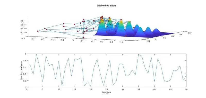
• In the above result, the red dots shows no. of points or coordinates of x, y under consideration for each iteration . large no. of red dots show values of coordinates of x, y varies each time iteration runs.
• Above plot of fopt vs iteration shows optimum value of function, fopt varies each time iteration runs. It also shows large variations in fopt values of each iteration. The large variations are result of not providing any bound to function.

Study 2 Statistical Behaviour with upper and lower bounds:

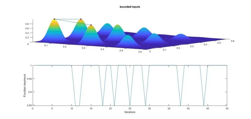
• The above result shows coordinstes of x, y are converging that of previous case. No. of red dots are less showing values of x and y are not varying much as in previous case.
• The bounds are provided, the value of function varies only in prescribed limits.

Study 3 Statistical behaviour with increasing GA iterations:

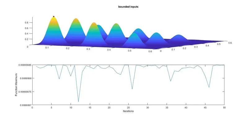
• After providing upper and lower bounds and options, it seems that the value of coordinates x,y converges to only one value for each iteration
• Value of x = 0.0668 & y = 0.0668
• The value of fopt comes out be nearly 1.

REFERANCES:

https://in.mathworks.com/help/gads/how-the-genetic-algorithm-works.html

https://in.mathworks.com/help/gads/ga.html#mw_f69991d0-5b23-4023-8c8e-e2890f2474d5

https://skill-lync.com/knowledgebase/genetic-algorithm-explained