Week 3 - Solving second order ODEs

AIM: To write a program in MATLAB that will simulate the pendulum motion.

OBJECTIVE:

• To solve the given ODE that represents the equation of motion of a simple pendulum.

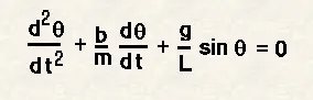
Where, g = gravity in m/s^2,

L = length of the pendulum in m,

M = mass of the ball in kg,

B = damping coefficient.

• From the results of ODE animate the motion of the pendulum.

GIVEN DATA:

L = 1 metre,

m = 1kg,

b = 0.05,

g = 9.81m/s^2

angular velocity = 3rad/sec at t = 0

time span = 0 – 20sec

THEORY AND CALCULATIONS:

In given equation,

Let us consider,

θ = θ1............(1)

dθ/dt = dθ1/dt = θ2............(2)

d^2θ/dt^2 = dθ2/dt..........(3)

By using above constants, the second order differential equation becomes,

dθ2/dt = -(b/m)θ2 – (g/l)sinθ

Writing above equation in form of matrix

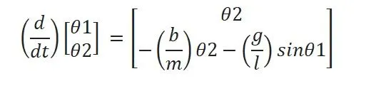
Using the above equation and ode45 solver we can solve the equation and animate the simple pendulum in MATLAB

Note:

• Ode45 solver is an inbuilt solver in MATLAB. The ode45 solver requires simple differential equation to solve any kind of higher order differential equation.
• The given equation is of order 2 so i simplified it in simple ODE to use ode45 which is developed on basis of Runge-kutta method to solve higher order differential equation.
• Syntax of ode45 solver

[t,results]=Ode45(@(t,theta) ode_func(t,theta,b,g,l,m),t_span,theta_0)

MATLAB Code:

clear all
close all
clc

%inputs
b = 0.05;
g = 9.81;
l = 1;
m = 1;

% Initial Condition
% angular displacement is 0 and angular velocity is 3rad/sec
theta_0 = [0;3];

% time points
%pendulum oscillates between 0-20 seconds 
t_span = linspace(0,20,200);

% solving ODE using ode45 function
[t,results] = ode45(@(t,theta) ode_func(t,theta,b,g,l,m),t_span,theta_0);

%plotting of angular velocity and displacement
figure(1)
plot(t,results(:,1))
hold on
plot(t,results(:,2))
title('motion of pendulum')
ylabel('displacement vs angular velocity')
xlabel('time')
legend('displacement','angular velocity')
grid on


% Starting loop to get animation
ct = 1;
for i = 1:length(t_span)
    figure(2)
   

    %fixed coordinates of one end of pendulum
    x0 = 0;
    y0 = 0;

    %moving coordinates (bob)
    x1 = l*sin(results(i,1));
    y1 = -l*cos(results(i,1));

    %plotting the animation
    figure(2)
    plot([x0 x1],[y0 y1],'linewidth',3,'Color','b')
    hold on
    plot(x1,y1,'o','markersize',15,'MarkerFaceColor','r')
    plot([-3 3],[0 0],'LineWidth',2,'Color','g')
    hold off
    title('motion of pendulum')
    axis([-3 3 -2 2])
    grid on
    
    
    M(ct) = getframe(gcf);
    ct = ct+1;
  
end

% Animation of pendulum
movie(M)
videofile = VideoWriter('pendulum_animatin.avi');
open(videofile)
writeVideo(videofile,M)
close(videofile)

Function Code(ode_func):

function [dtheta_dt] = ode_func(t,theta,b,g,l,m)
theta1 = theta(1);
theta2 = theta(2);
dtheta1_dt = theta2;
dtheta2_dt = -(b/m)*theta2-(g/l)*sin(theta1);
dtheta_dt = [dtheta1_dt;dtheta2_dt];
end

OUTPUT:

the following plot obtained by the given data.

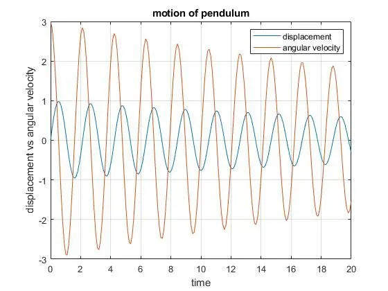
• The plot is drawn between angular acceleration and displacement of motion of simple pendulum
• The blue curve is displacement and red is angular velocity as shown in legend.
• At the end both velocity and diplacement becomes zero and pendulum comes in rest.

CONCLUSION:

we have animated the simple pendulum by the given data and ode45 solver.

ANIMATION LINK:

https://youtu.be/s5lh02sB0m0