Project 2 - Rankine cycle Simulator
AIM: To simulate the Rankine Cycle and plot the corresponding T-S and H-S plots using MATLAB.
OBJECTIVE:
- Calculate the state points of the Rankine Cycle based on given inputs.
- Plot the corresponding T-S and H-S plots for the given set of inputs.
GIVEN:
Input Values:
- Turbine Inlet temperature = 400 deg Celsius
- Turbine Inlet pressure = 30 bars
- Turbine Outlet Pressure = 0.05 bars
- Condenser Inlet Pressure = 0.05 bars
Required Output values:
- Net work output
- Back work ratio
Note: “The standard XSteam library is used to get the steam table data for water is given, which is used to calculate the points in between the state variables.”
THEORY:
Introduction to Rankine Cycle:
The Rankine cycle is an idealized thermodynamic cycle describing the process by which certain heat engines, such as steam turbines or reciprocating steam engines, allow mechanical work to be extracted from a fluid as it moves between a heat source and heat sink.
The Rankine cycle closely describes the process by which steam engines commonly found in thermal power generation plants harness the thermal energy of a fuel or other heat source to generate electricity. Possible heat sources include combustion of fossil fuels such as coal, natural gas, or oil, renewable fuels like biomass or ethanol, nuclear fission, and concentrated solar power. Common heat sinks include ambient air above or around a facility and bodies of water such as rivers, ponds, and oceans.
The ability of a Rankine engine to harness energy depends on the relative temperature difference between the heat source and heat sink. The greater the differential, the more mechanical power can be efficiently extracted out of heat energy, as per Carnot's theorem.
The efficiency of the Rankine cycle is limited by the high heat of vaporization of the working fluid. Unless the pressure and temperature reach super critical levels in the boiler, the temperature range that the cycle can operate over is quite small: Steam turbine entry temperatures are typically around 565 °C and condenser temperatures are around 30 °C. This gives a theoretical maximum Carnot efficiency for the turbine alone of about 63.8% compared with an actual overall thermal efficiency of less than 50% for typical power stations.
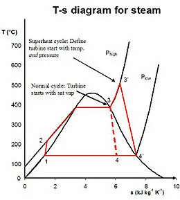
Rankine engines generally operate in a closed loop where the working fluid is reused. The water vapour with condensed droplets often seen billowing from power stations is created by the cooling systems (not directly from the closed-loop Rankine power cycle). This 'exhaust' heat is represented by the "Qout" flowing out of the lower side of the cycle shown in the T–S diagram below.
Processes in the Rankine cycle:
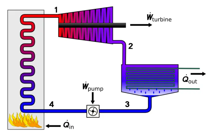
There are four processes in the ideal Rankine cycle.
Process 1-2 is isentropic compression: The working fluid is pumped from low to high pressure. As the fluid is a liquid at this stage, the pump requires little input energy
Process 2-3 is constant pressure heat addition in boiler. The high-pressure liquid enters a boiler, where it is heated at constant pressure by an external heat source to become a dry saturated vapour. The input energy required can be easily calculated graphically, using an enthalpy–entropy chart (h–s chart, or Mollier diagram), or numerically, using steam tables or software.
Process 3-4 is isentropic expansion. The dry saturated vapour expands through a turbine, generating power. This decreases the temperature and pressure of the vapour, and some condensation may occur. The output in this process can be easily calculated using the chart or steam tables as noted above.
Process 4-1 is constant pressure heat rejection in condenser. The wet vapour then enters a condenser, where it is condensed at a constant pressure to become a saturated liquid.
Procedure:
- First, all the required variables and parameters were found out to calculate.
- Then, using the ‘XSteam’ library function, all the parameters were sorted out.
- Then, the usual calculations and plotting of graphs were done as per the theory of thermodynamics.
MATLAB Code:
close all
clear all
clc

% Displaying rankine cycle simulator and its processes
disp('              RANKINE CYCLE SIMULATOR')
fprintf('\n 1-2 is the isentropic expansion in the Turbine')
fprintf('\n 2-3 is the constant pressure heat rejection by the Condenser')
fprintf('\n 3-4 is the isentropic compression in pump')
fprintf('\n 4-1 is the constant prressure heat addition by the boiler\n')

% Inputs
fprintf('\n ENTER INPUTS')
p1 = input('\nEnter the pressure at turbine Inlet(Bar): ');
t1 = input('Enter the Temperature at turbine Inlet (Celsius): ');
p2 = input('Enter the pressure at the Turbine Outlet(Bar): ');

% variable at state point 1
h1 = XSteam('h_pt',p1,t1);        %Enthalpy
s1 = XSteam('s_pt',p1,t1);        %Entropy
hf1 = XSteam('hL_p',p1);          %Enthalpy of saturated liquid
hg1 = XSteam('hV_p',p1);          %Enthalpy of saturated vapour
ts1 = XSteam('Tsat_p',p1);        %Saturation Temperature
sf1 = XSteam('sL_p',p1);          %Entropy of saturated liquid
sg1 = XSteam('sV_p',p1);          %Entropy of saturated vapour

% variables at state point 2
s2 = s1;
sf2 = XSteam('sL_p',p2);
sg2 = XSteam('sV_p',p2);
x = (s2 - sf2)/(sg2 - sf2);         % Dryness Factor
hf2 = XSteam('hL_p',p2);
hg2 = XSteam('hV_p',p2);
h2 = hf2 + x*(hg2-hf2);
t2 = XSteam('T_ph',p2,h2);
ts2 = XSteam('Tsat_p',p2);

% variables at state point 3
h3 = hf2;
s3 = sf2;
t3 = t2;
p3 = p2;

% variables at state point 4
p4 = p1;
s4 = s3;
h4 = XSteam('h_ps',p4,s4);
t4 = XSteam('T_ps',p4,s4);

t = linspace(0,374,500);        % temperature space for plotting saturation curve

% plotting T-S Diagram
figure(1)
hold on
% plotting saturation curve
for i = 1:length(t)
    plot(XSteam('sL_T',t(i)),t(i),'.','Color','b')
    plot(XSteam('sV_T',t(i)),t(i),'.','Color','b')
end

% plotting cycle
plot([s1 s2],[t1 t2],'linewidth',2,'Color','r')
if x>1
    t3 = Ts2;
    plot([s2 sg2 s3 s4],[t2 ts2 t3 t4],'LineWidth',2,'Color','r')
    T2 = Ts2;
else
    plot([s2 s3 s4],[t2 t3 t4],'LineWidth',2,'Color','r')
end
l = linspace(t1,t2,1000);
for i = 1:length(l)
    plot(XSteam('s_pT',p1,l(i)),l(i),'.','Color','r')
end
plot([sf1 sg1],[ts1 ts1],'LineWidth',2,'Color','r')
xlabel('Entropy[KJ/Kg-K]')
ylabel('Temperature[K]')
title('T-S Diagram')

% plotting H-S Curve
figure(2)
hold on
% plotting Saturation curve
for i = 1:length(t)
    plot(XSteam('sL_T',t(i)),XSteam('hL_T',t(i)),'.','Color','b')
    plot(XSteam('sV_T',t(i)),XSteam('hV_T',t(i)),'.','Color','b')
end

% Plotting Cycle
plot([s1 s2 s3 s4 s1],[h1 h2 h3 h4 h1],'LineWidth',2,'Color','r')
xlabel('Entropy[KJ/Kg-K')
ylabel('Enthalpy[KJ/Kg')
title('H-S Diagram')

% Calculations
W_turbine = h1-h2;          % Turbine work
W_pump = h4-h3;             % Pump work
Q_in = h1-h4;               % Heat added
Q_out = h2-h3;              % Heat rejected
W_net = W_turbine - W_pump; % Net work done
N_therm = (W_net/Q_in)*100; % THermal Efficiency
SSC = 3600/W_net;           % Specific steam consumption
BWR = W_pump/W_turbine;     % Back work ratio

% printing results
fprintf('\n\nRESULTS\n')
fprintf('At state point 1:\n')
fprintf('P1 is : %.2f bar\n',p1)
fprintf('T1 is : %.2f Deg Celcius\n', t1)
fprintf('H1 is : %.2f KJ/Kg\n',h1)
fprintf('S1 is : %.2f KJ/Kg-K\n',s1)


fprintf('\nAt state point 2:\n')
fprintf('P2 is : %.2f bar\n',p2)
fprintf('T2 is : %.2f Deg Celcius\n', t2)
fprintf('H2 is : %.2f KJ/Kg\n',h2)
fprintf('S2 is : %.2f KJ/Kg-K\n',s2)

fprintf('\nAt state point 3:\n')
fprintf('P3 is : %.2f bar\n',p3)
fprintf('T3 is : %.2f Deg Celcius\n', t3)
fprintf('H3 is : %.2f KJ/Kg\n',h3)
fprintf('S3 is : %.2f KJ/Kg-K\n',s3)

fprintf('\nAt state point 4:\n')
fprintf('P4 is : %.2f bar\n',p4)
fprintf('T4 is : %.2f Deg Celcius\n', t4)
fprintf('H4 is : %.2f KJ/Kg\n',h4)
fprintf('S4 is : %.2f KJ/Kg-K\n',s4)

fprintf('\nWork done by turbine is : %.2f KJ/Kg\n',W_turbine)
fprintf('Pump Work is : %.2f KJ/Kg\n',W_pump)
fprintf('Net Work Done is : %.2f KJ/Kg\n',W_net)
fprintf('Thermal Efficiency is : %.2f percent\n',N_therm)
fprintf('S.S.C. is :%.2f Kg/KWh\n',SSC)
fprintf('Back Work Ratio is : %.3f \n',BWR)
Steps to program:
- The first step is to make provision for MATLAB to accept user input. Input() command is used to provide the user inputs
- Now, based on the user inputs the four parameters of rankine cycle are calculated.
- Thermodynamic parameters like H,S,T,P and dryness factor x at state point 2 is calculated using the XSteam Matlab program provided.
- After calculating all parameters, the next objective is to calculate pump work, turbine work, net work output, back ratio and thermal efficiency.
- All these results are displayed in the command window using fprintf command.
- The next objective is to plot the graph for H-S and T-S. The first step in plotting the graph is to plot the saturation curve which is plotted using for loop. Under for loop, values for entropy and enthalpy are calculated over a temperature range and other processes are plotted by plotting respective values of H,S,T.
- Now, when the program runs it asks the user to enter inputs, Turbine Inlet temperature, Turbine Inlet pressure and turbine outlet pressure.
- After the input parameters are given, results are displayed in the command window.
Results:
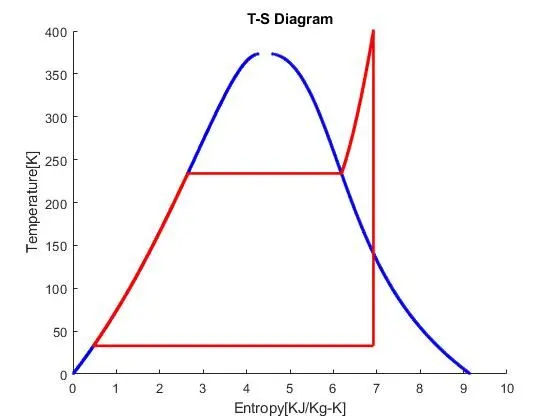
Input parameters in the command window:
- Turbine Inlet temperature = 400 deg Celsius
- Turbine Inlet Pressure = 30 bars
- Turbine Outlet Pressure = 0.05 bars = Condenser Inlet Pressure
DIAGRAMS:
1) T-S plot
2) H-S plot
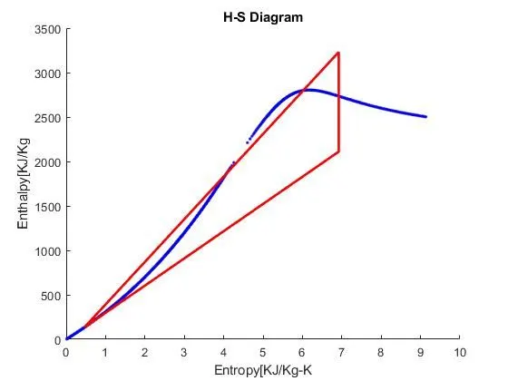
Note: Here in both the plots the blue curve represents saturation curve and red curve represents the cycle.
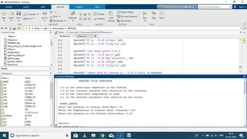
Command Window:
 RANKINE CYCLE SIMULATOR

 1-2 is the isentropic expansion in the Turbine
 2-3 is the constant pressure heat rejection by the Condenser
 3-4 is the isentropic compression in pump
 4-1 is the constant prressure heat addition by the boiler

 ENTER INPUTS
Enter the pressure at turbine Inlet(Bar): 30
Enter the Temperature at turbine Inlet (Celsius): 400
Enter the pressure at the Turbine Outlet(Bar): 0.05


Results
At state point 1:
P1 is : 30.00 bar
T1 is : 400.00 Deg Celcius
H1 is : 3231.57 KJ/Kg
S1 is : 6.92 KJ/Kg-K

At state point 2:
P2 is : 0.05 bar
T2 is : 32.88 Deg Celcius
H2 is : 2110.71 KJ/Kg
S2 is : 6.92 KJ/Kg-K

At state point 3:
P3 is : 0.05 bar
T3 is : 32.88 Deg Celcius
H3 is : 137.77 KJ/Kg
S3 is : 0.48 KJ/Kg-K

At state point 4:
P4 is : 30.00 bar
T4 is : 32.95 Deg Celcius
H4 is : 140.76 KJ/Kg
S4 is : 0.48 KJ/Kg-K

Work done by turbine is : 1120.86 KJ/Kg
Pump Work is : 3.00 KJ/Kg
Net Work Done is : 1117.87 KJ/Kg
Thermal Efficiency is : 36.17 percent
S.S.C. is :3.22 Kg/KWh
Back Work Ratio is : 0.003
Screenshot Of OUTPUT screen
Conclusion:
Net work Output = 1117.87 KJ/Kg
Back work Ratio = 0.003
Referances: