Week 7 State of charge estimation
1.Simulate the 3 test cases from harness dashboard and write a detailed report on the results
2.What is coulomb counting? Refer to the above model and explain how BMS implements coulomb counting for SOC estimation?
AIM: -
- To simulate the Simulink model of a lithium-ion battery management system for 3 test cases and to explain the results.
- To explain coulomb counting and it’s use in estimating the state of charge of a battery pack of the above model.
- Simulate the 3 test cases from harness dashboard and write a detailed report on the results: -
To know about the test cases, we have to know about the simulation of the lithium-ion Battery Management System (BMS) it working plant and also BMS ECU (Electronic Control Unit) which is the software simulation environment.
Battery management system (BMS):
The Battery Management System is a system which is used to predict the health and capacity of the charge in the battery. It is an electronic control circuit that monitors and regulates the charging and discharging of batteries. It is also used to know that indicating the remaining time or value which is used to use. The main use of the BMS is the safety purpose that to not to reach over currents and voltage and also the temperature.
The BMs not only monitors the values but also for the detection of battery type, voltages, temperature, capacity, state of charge, power consumption, remaining operating time, charging cycles, and some more characteristics. By this simulation BMS model we can also balance the model by using balance logic which present in the BMS ECU.
The simulation of the BMS model can be download through the link given below.
After down loading the model by using some steps we can use the simulation model in the MATLAB which are seen in FAQ from the (battery management system Design Week 7 Session 3 part 2)through
- Simulation of BMS model in simulink
Now the model of the BMS simulation is look like as shown below. Which named in the downloads are BMS_closedloop
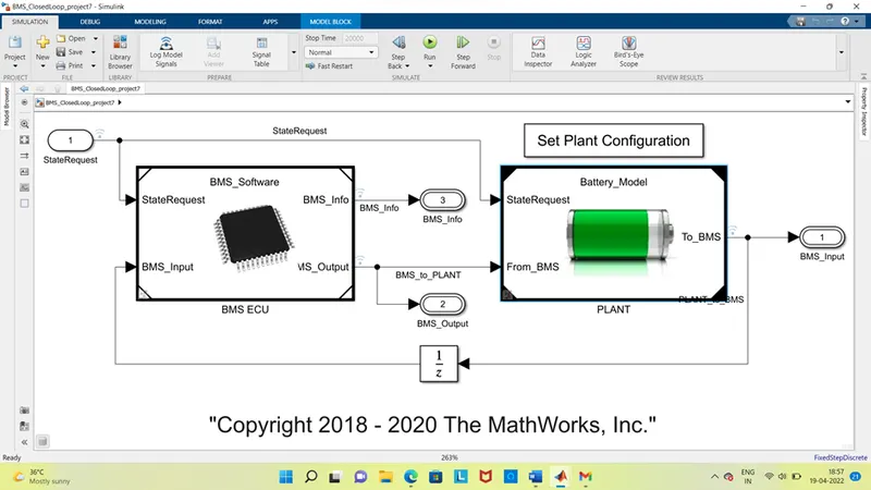
The BMS model is a combination of various subsystem models. The models that we consist of 3 parts are,
- The BMS ECU.
- BMS plant. And,
- The test hardness Dashboard.
BMS Plant:
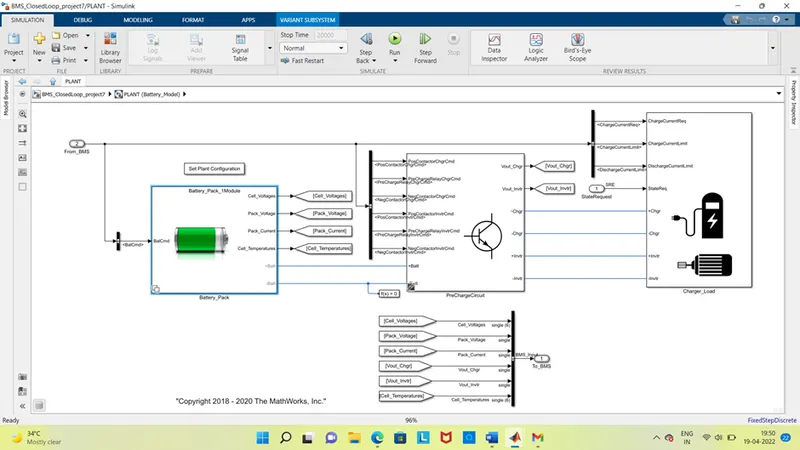
by clicking on the plant sub system in the BMS model we can get this BMS plant which look like as shown.
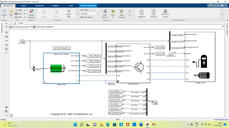
From this plant sub system, we can observe the main parts are, battery pack, pre charge circuit, charger load and their internal connections as closed loop for the feedback purpose.
The battery pack in the plant model having the input as balance command from the BMS and have the outputs as cell level voltage, total pack voltage, total pack current, cell temperatures and battery +ve and -ve terminals.
The inner subsystem or parts or the blocks in the battery pack are which look like as shown.
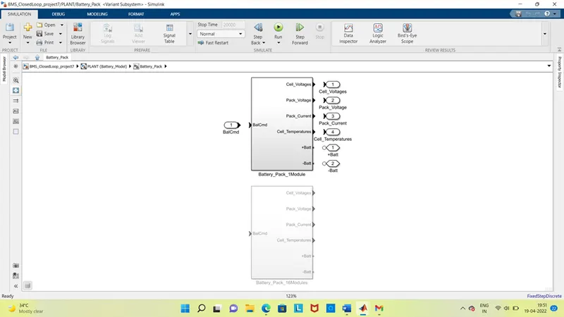
It mainly consists of two types those are battery pack 1module which having 6 cells in the 1 module that connected in series to each other which have 6 +ve terminals of each cell and 1 -ve terminals which goes to ground. By this series connection the voltage in each cell is calculated as total pack voltage and the current remains same.
The other type is having the battery pack 16modules which having 16 modules connected to the battery pack of each having the 6 cells which all are connected In series so the total cells are 96 connected in series to each other in this also having the cell level voltage, pack voltage and the pack current cell temperature is calculated for each cell in 1 and 16 module.
This battery and the cell +ve and-ve terminals are connected to the pre charger circuit which is connected between the charge or load and battery to not to affect by over charge and over current which is act as a transistor. The inner part of the pre charger circuit is looks as shown,
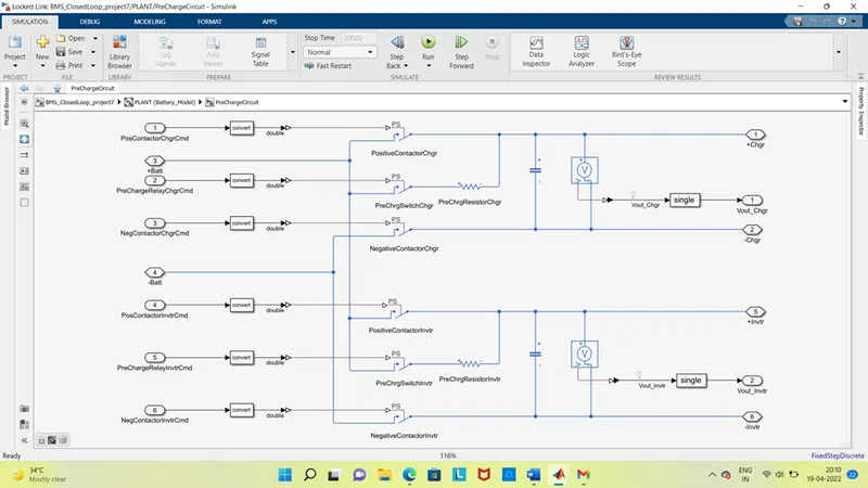
If we observe here that pre charger switching charge is connected in between the positive and negative contactor charger with the pre charge resistor in the charge side. As the same in the inverter side also the pre charger is connected between positive and negative contactor through resistor. Based on the given condition the charger or the inverter are connected through the resistor. When they connected first the negative contactor is connected then it flows to the pre charged switch after that it flows to positive contactor charge through the high levelled resistor for the time delay operations if there is any fault observed in this circuit the pre charge is disconnects and it cut off with the positive contactor for the protection purpose.
The next one is the charger load which is used to connect to the battery for charging through the charger and to discharge through the load. The inner part of the charger load having the charger and the driver load with their internal connections connected in parallel. Based on the given state request the connections are made and there connect respectively. The blocks of the inner circuit of the charger load look like as shown,
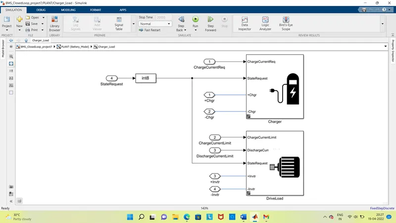
BMS ECU:
The full form of BMS ECU is Battery Management System Electronic Control Unit. It is a simple BMS software which is used to run the battery functionalities with out errors. These functionalities or the programmes are implemented at state machine diagram which is placed in the BMS ECU which is looks like,
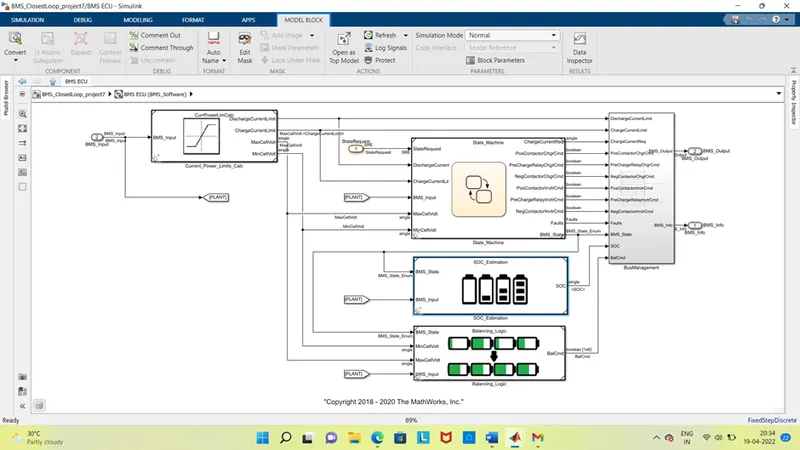
In this as we can see that the main parameters were the current power limits calculator, state machine, SOC estimation, Balancing logic, bus management.
From all the parameters the state machine is the main part which is be the brain system or function of the BMS ECU.
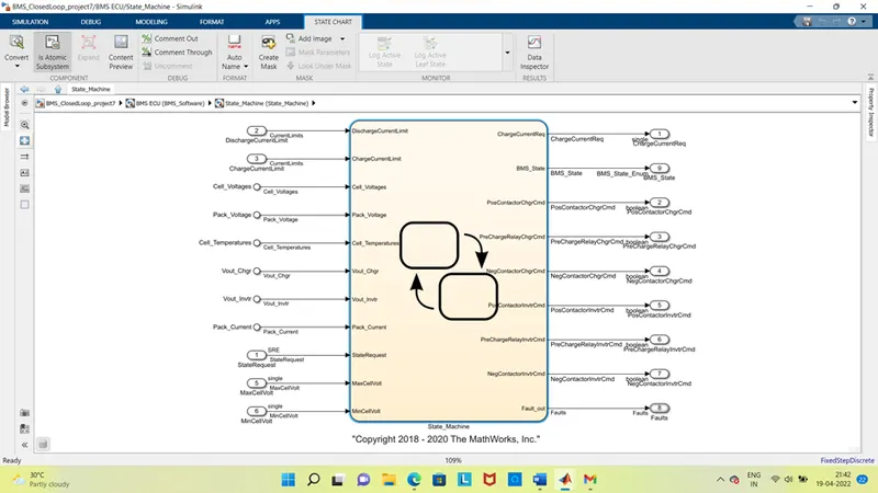
As the name it self indicates that it works as the brain that is it takes the decision of controls state od BMS, faults detections, its internal conditions etc. it takes the inputs as current limits, cell and pack voltages, cell temperatures, charger and inverter voltage outputs, pack current, state request, max and min cell voltages. After the logical operations or algorithm functions are completed based on the given inputs the output is taken from other side of the state machine those are, required charge current, BMS state, pre charge relay charger and inverter command, positive contractor charger and inverter command, negative contractor charger and inverter command, fault outputs. It is used to calculate the charge and dis charge currents based on the given inputs.
The flow chart of the state machine is as below,
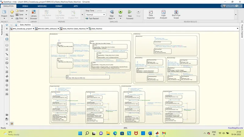
As from the above flow chart we can observe that how a state machine works. For every work there been a sperate blocks like main state machine, for fault monitoring, for charge contactor state and for inverter contactor state.
As the same to calculate the state of charge (SOC) with the exact estimation we consider the SOC Estimation system which is placed at the bottom of the state machine subsystem. The inner blocks of this system look like,
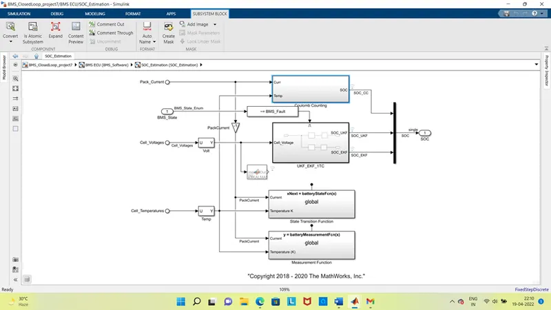
Here by using the pack current, cell voltage and cell temperature we are finding the SOC. He SOC are found by three types those are coulomb counting and SOC UKF and EKF which all are connected to the output SOC through bus selector.
For the balancing the battery cells with out causing any errors or short circuits which leads to destroy the total battery pack functions, we use the balancing logic system which inner system is as below.
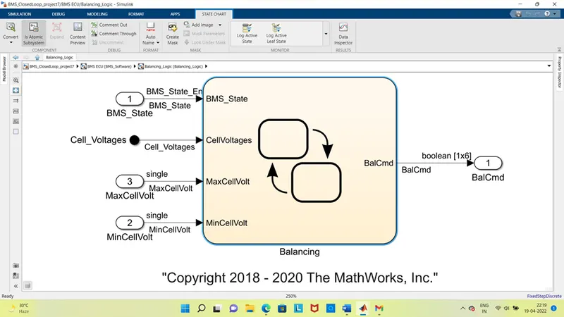
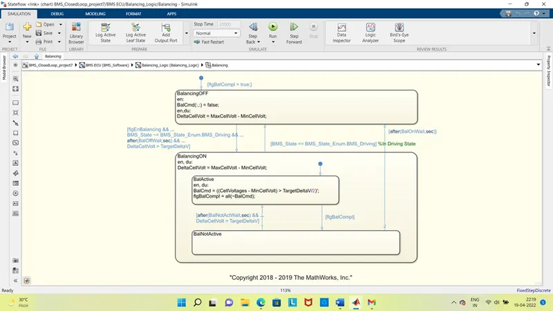
If we observe here that in the flow chart we can identify the balancing conditions how to balace the battery when it gets fault occurs.
From the above graph we can know that if any fault or false statement that the max and min cell voltage or cureent exceed or reduced from the limits it get start condut to balancing that is balancing on, if the measured values are in the limits only then it be in off condition only. If any fault occurs its get to the specified cell and rectify the problem and be place the value to the mean value of all the cells and gets to off state.
The calculated values from the state machine, SOC and balancing commands are passed through a bus management system through bus selector which is then relayed to the BMS plant output and info.
test hardness Dashboard:
the test hardness dashboard is the model which is used to test the BMS model outputs by changing the values of the given input to the BMS. By changing the values of the test conditions, we can observe the results in the form of the graph in the scope.
The model of the test hardness model is as shown below,
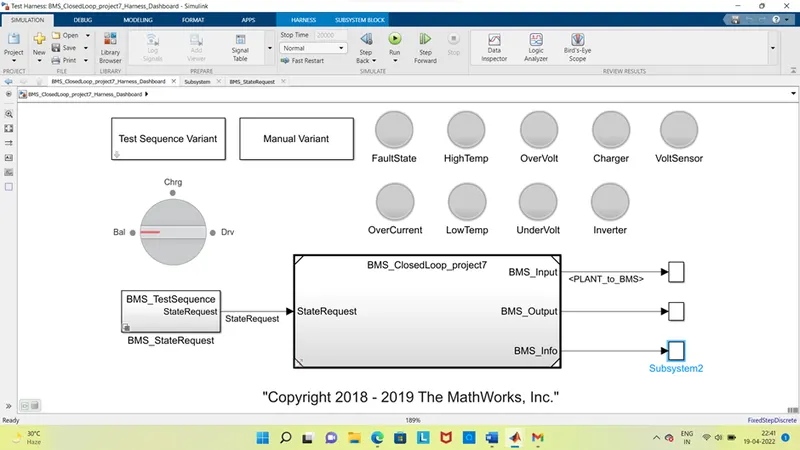
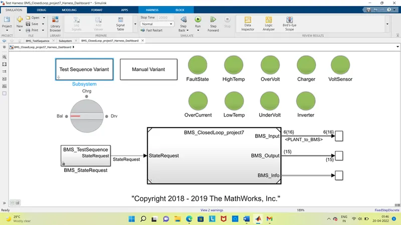
In this model if we observe the lights which are in the green colour used to indicated the faults conditions, when any faults are occurred in the model by the given input these led lights blink in the red coloured which indicates fault state. the faults that are detecting in this model are, fault state, over current, high temperature, low temperature, over voltage, under voltage, charger, inverter, volt sensor.
There are three operating conditions in this model which the battery run in these 3 operations when it is on those are driving, charging and balancing.
There are 3 test case conditions in this model, which is used to find out the results those are chose by the test sequence variant sub system which look as shown,
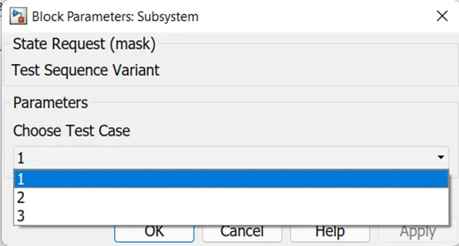
By clicking on any of these 3 test cases the inputs are given. We can see this in the BMS state request by clicking on the BMS test sequence. Let's get in to the test conditions by running with 20000sec.
Test condition 1
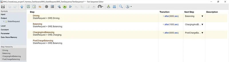
From the above fig we can say that the simulation is running for 20000 seconds. Here For 3000 seconds the vehicle is in driving condition, after that is from 3001 to 4000 seconds that is (1000 sec) the BMS is running the balancing condition and finally from 4001 to 9000 seconds (5000 sec) the BMS is charging the battery and starts balancing again from 9001 to 20000 seconds (11000 sec).
By clicking on the run by keeping the stop time to 20000 sec in the simulation we can get the results in the scope as a graph and the test hardness model which looks like as shown,
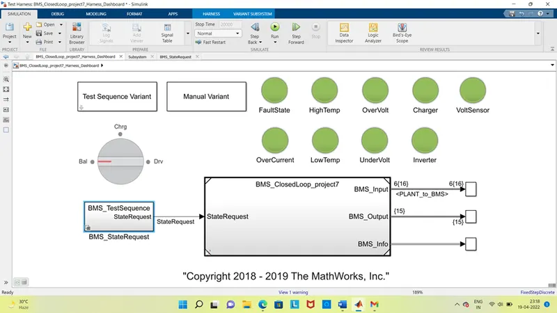
Here if we observe that the LED lights indicate all in green only that there are no issues in the model so the simulation ran without fault and it remains same.
The graphical representation of the given condition is given below,
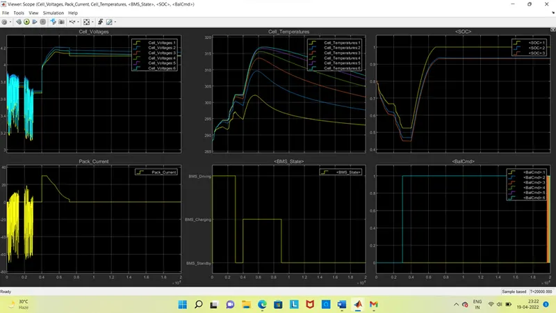
The graphs that are given or plotted in the fig are cell voltages, pack current, cell temperature, BMS state, state of charge and balance command.
If we observe the cell voltages graph each cell is indicated by the different colour for the identification. As the same the cell temperatures are given for each cell as the same is given to the balance command. If we observe in the SOC graph, we can see the different indications which are given for the coulomb counting and SOC UKF and EKF SOC conditions.
here the voltages of each cell were different because of their construction or by any other reasons. But there are been in the given input limits which are given in state machine sub system. Here if we observe from 0 to 3000 sec the voltage in fluctuates that is up and down from the 3.9 to 3.1 V which is their discharge limits. These are plotted due the driving condition. From 3001 to 4000 sec, it is in balance condition hence it is in constant state at 3.6 to 3.9V. after that from 4001 to 9000 sec the state was the charging state. at this condition the constant current (CC) and constant voltage (CV) are occur, at start CC are with very less time after that CV occur for the time longer than the CC. after charging was completed it changes to balance condition due to the balancing system. From 9001 to 20000 sec again the condition was the balancing condition due to this it remains constant up to 20000 sec.
if we observe the current graph. The fluctuations are occurred due to driving condition from 0 to 3000 sec it is from 20A to -65A here -ve indicates reverse direction. from 300 to 4000 sec the balancing is placed due to this the current is located at 0 value. Now from 4001 to 9000 sec it gets charging due to this at stat it was CC hence it kept constant at range of 30A after the CC it gets CV which it starts decreasing to 0A. after 9000 sec due to the balancing condition it again placed in the 0A value up to 20000 sec.
if we observe in the cell temperature, we can observe different temperatures for differen cell due to the location in the battery pack and also their construction. If we observe here that in driving condition the temperature increased based on the driving conditions, but in the balance condition it gets tried to slow down which is going to cooling their range. Again, in the charging condition it reaches to the highest ranges which we can conclude that in charging that batteries get more heat. Again, after balancing condition, it reduces its temperature and tries to gets normal.
In the BMS state it is simple to understand that when the state is getting activated it gets in the constant after that it getting to 0. If we see here in the starting the driving is on up to 3000 sec after that the balancing takes place stand by is on. When charging is going BMS charging is on and again for balancing the stand by in getting on
In the SOC graph the coulomb counting is different and SOC UKF and EKF SOC conditions are plotted as near to each other in this the coulomb counting is little high but the SOC UKF and EKF are perfect or accurate than coulomb. If we observe the graph that the battery SOC is at the range of 80% at the starting. Due to driving the discharge of the battery occur and it reduced to 45 to 50%, in balancing condition it remains constant. Now due to charging occurred it started charging if we observe here at staring stage of charging it gets charged faster after that it takes due to CC and CV respectively. When it gets charged it takes the constant position from 7000 to 9000 sec. after that due to balancing condition it again in the constant mode.
Here in the balance command graph due to changes in the cells the balancing values are changed to keep the mean cell value to constant.
Test Condition 2
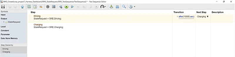
In the second test condition there is only driving and charging phase that is from 20000 sec, where 10000 sec for driving that is the vehicle is in driving condition and from 10001 to 20000sec the vehicle is in charging condition. By clicking on the run by stop time 20000 sec we get the results in the test hardness is,
If we observe here that the test model is not changed also the faults are not detected because all the lights are glowing in green only.
The graphical representation of the results in the test hardness model are,
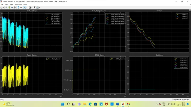
If we observe here that the graph stops at 8692 sec due to it battery is fully discharged.
In the voltage that the varies from 3.V to 3.02V which continually discharged from 0 to 8692 sec.
In the current graph if we see that the value varies from 20A to -70A due to reverse direction the negative sign is assigned. For constant value it reaches to 0
In the temperature graph the values raises nearly from 290 to 322 which is reaches to max temperature range
In the BMS state the line is placed only in the driving condition only because the battery is off in the driving condition only.
If we observe the SOC graph, we can see that the coulomb counting and SOC UKF and EKF are discharged to zero from 80% but the coulomb counting shown some value but it not exact.
In the balance command the data is placed in the line of 0 which is the balance condition is in off condition in entire run.
Test condition 3
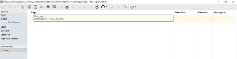
This condition is only to study the cell charging during the simulation of 20000 sec. the test hardness model does not have any changes and it remains same as shown below, and the led lights also glowing in green colour.
The graphical representation of the cells and battery pack results are shown below.
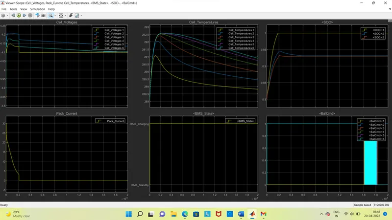
If we observe here that we only given the charging in the model as an input for the 20000 sec.
The voltage in the graph is raises from 4.1V to 4.2V very quick due to CC then after that due to the CV it takes time to charge with CV after that fully charged it gets been constant with 4.1V up to 2000 sec.
If we see the current graph that it raises to 30A in the CC time. After that in the CV time it gets reduced to minimum value and then it gets to 0A due to it reached the fully charged condition.
In cell temperature at CC an CV the temperature raises immediately at CC and increased little slow at CV. When the battery pack get fully charged it start reducing the temperature but it is in the limited ranges only.
In the BMS state the value shown the line in the charging because we using the charging for the entire 20000 sec.
In the SOC graph the values changes from 80% to 100% because it already has the charging value of about 80%. After getting the value to the max charge condition the value remains constant in the battery pack.
In the balancing command the values are plotted based on the values of the cell in the voltages. By changing the values which changed out of range it starts balancing and again it gets off when it reached to limit values.
- What is coulomb counting? Explain how BMS implements coulomb counting for SOC estimation?
Coulomb Counting:
The coulomb counting method is also known as the battery current integration method. In this method, a discharging/charging current I(t) is measured and integrated over the period of time to calculate the amount of energy remaining inside the battery. This coulomb counting is used to calculate the SOC in the Battery Management System which gives accurate values but not much than Kalman Filter.
For the calculation of this method, we use the equation in terms of SOC was,
`OC(t)= SOC(t-1).∫_(t-1)^t▒(It.η)/Qn.d`
Were,
SOC(t-1) = Previous SOC value.
t = current or present time step.
t-1 = previous time step.
η = efficiency.
It = Discharge current.
Qn = charge capacity.
As we know that the State of Charge (SOC) is a parameter which is used to observe the battery and to represent the amount of energy that present in the battery with respect to total charged condition. The output of the SOC will give us that exact values that battery usage of energy at each point. But to calculate the output the SOC not have any direct method to implement in the MATLAB Simulink. For this we use some methods which gives the accurate values of SOC of the Li-ion battery, those are coulomb counting, fuzzy logic method, Kalman Filter method and some other. but in this above model we used the coulomb counting and the Kalman Filter methods.
To calculate the SOC, we use the SOC Estimation sub system which is used to calculate the coulomb counting and the Kalman Filter methods by using some blocks which as shown below,
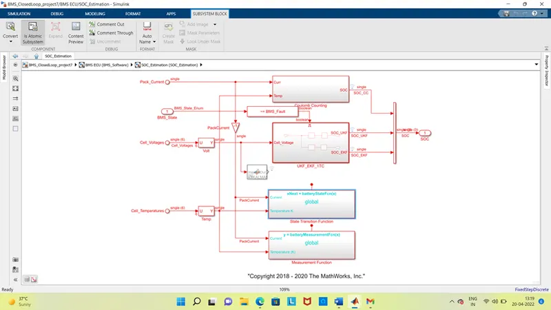
From here by clicking on the coulomb counting we will the design model of the coulomb counting which look like as below,
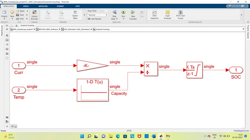
If we observe here that for the current integration, we used the Discrete time integrator which is implemented in the Z transform which also called as Z domine. it is used to connect with the SOC to give the output that the amount of energy remains in the battery that is battery capacity. In this model with the current value, we also sending the temperature value as an input through the gain block and look up table respectively which is connected to divide block which is used to calculate the SOC through this time integrator.