Week-4 Challenge WOT Condition Part-2

Aim:

Use the power train block set to simulate the given conditions and plot the answers.

Objective:

1. What is the difference between mapped and dynamic model of engine, motor and generator? How can you change model type?
2. How does the model calculate miles per gallon? Which factors are considered to model fuel flow?
3. Run the HEV Reference Application with WOT drive cycle. Change the grade and wind velocity in the environment block. Comment on the results.
4. Keeping all other parameters same, compare the simulated results of hybrid and pure electric powertrains.

Powertrain block set:

Powertrain block set is used for designing and simulation of automotive and control engineering.it provides a standard model architecture that can be reused throughout the development process. by these reference application projects assembled from blocks and subsystems, we can use as a starting point to create our own power train models.

we can use it for design trade-off analysis and component sizing, control parameter optimization, and hardware-in-the-loop testing.

1. What is the difference between mapped and dynamic model of engine, motor and generator? How can you change model type?

Difference between mapped and dynamic model:

The power train block set provides two types of engine, motor or generator models as ‘mapped and dynamic’.

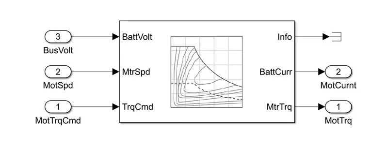
Mapped motor

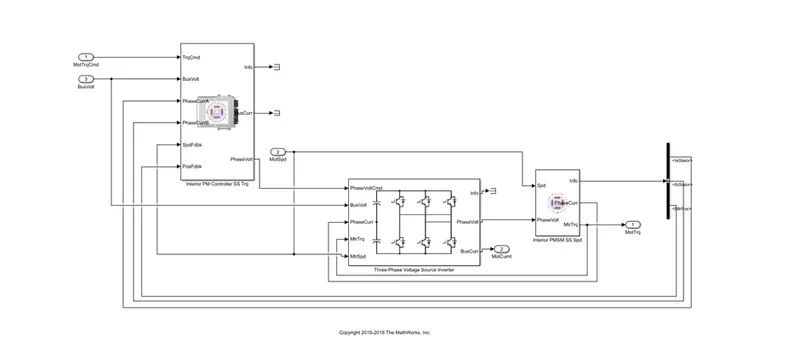
Dynamic motor

The main difference between mapped and dynamic model is,

The mapped is used the lookup table, steady-state lookup table for execution.

In case of motor /generator, specific electrical torque range with a torque-speed envelope or maximum motor power and torque.it also specify electrical losses as a single operating point that estimates losses across the operating range, measured loss or measured frequency.

In case of engine, the table provides overall engine characteristics including actual torque, fuel flow rate, bfsc, and engine-out exhaust emission.

• It uses a prebuilt data in look up table for the simulation of power train block set.
• In this the model calculations are very fast.
• Electric losses are needed to be specified if present.

In the dynamic model, it reduces the behaviour of component characteristics and are separated into lower-level components. By combining the components in this way, the model captures the dynamic effects.

In case of motor/generator, based on motor torque command, motor speed, we have to generate motor torque, motor current. For that we have used interior PM controller SS torque, 3-phase voltage source inverter, interior PMSM speed, type blocks.

In case of engine, we can see that dynamic blocks are required input, like torque command, engine speed etc data. So, to generate those input data we will use other blocks to generate data accordingly.

• It uses real time data for calculating every behaviour of vehicle characteristics like speed, velocity wheel braking, etc.
• In dynamic model the calculation is time consuming process.

Changing model type:

For changing the model from one form to another

Ex: to change the model from mapped to dynamic,

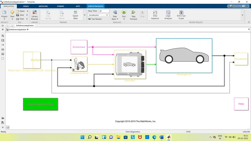
Open ‘EV Reference application’ in power train block set in getting started with powertrain block set through MATLAB help as shown in below fig.

After open the model be look like as below. It’s a everswe typr model from drive cycle to wheel.

It consists of drive cycle, environmental conditions, longitudinal driver controlers and passenger car, visualization.

Now open the passenger car block and select the electric plant block as shown below.

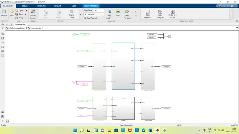
After that select the ‘motgenEVmapped’ block as shown.

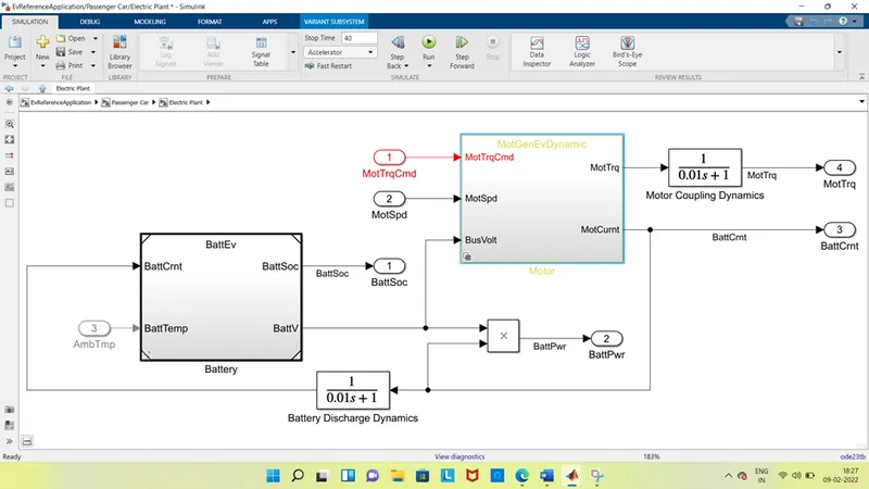
As shown the motgenEVmapped be selected.

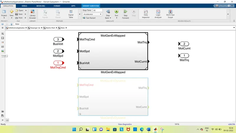
Now for changing mapped to dynamic block set, right click on the dynamic screen and select variant. Then click on ‘open in variant manager’. And block is looks like,

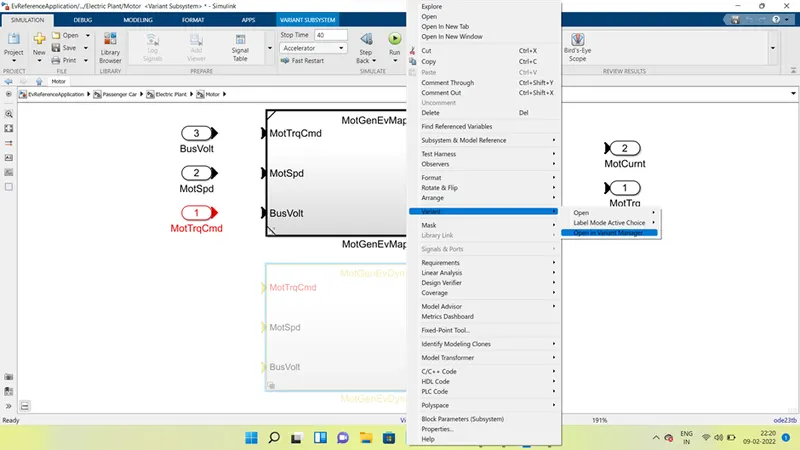
After clicking ‘open in variant manager’ the screen be as shown as below,

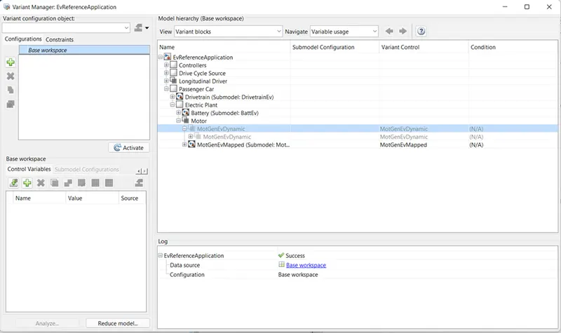
Now click on the ‘MotGenEVDynamic’ and select ‘set as label mode active choice’, after when we close the variant manager block it changes to dynamic block.

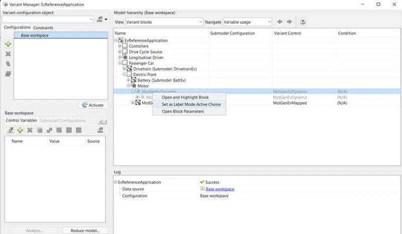
To change from dynamic model to mapped model same process be applied but instead of ‘MotGenEvDynamic’ choose ‘MotGenEvMapped’ in variant manager block.

2. How does the model calculate miles per gallon? Which factors are considered to model fuel flow?

Miles per gallon:

Gallon is a unit of measurement for liquids. miles per gallon is a fuel economy rating determined by how far a car can travel on a gallon of gasoline or diesel. Although the metric version would be kilometres per litre, MPG is adopted in many metric-system countries, like Canada.

I America it is equal to about 3.785 litres. MPG or miles per gallon, is a distance measured in miles, that a car can travel per gallon of fuel. It is also a primary measurement of a car’s fuel efficiency. The higher the car’s MPG, the more fuel efficiency in it.

Miles per gallon is generate by plotting ‘vehicle speed’ and battery power’ on graph,the vehicle speed can be seen by clicking on the model EvrRferenceApplication/ passenger car/ drive train(drive trainEV)/ vehicle.as shown.

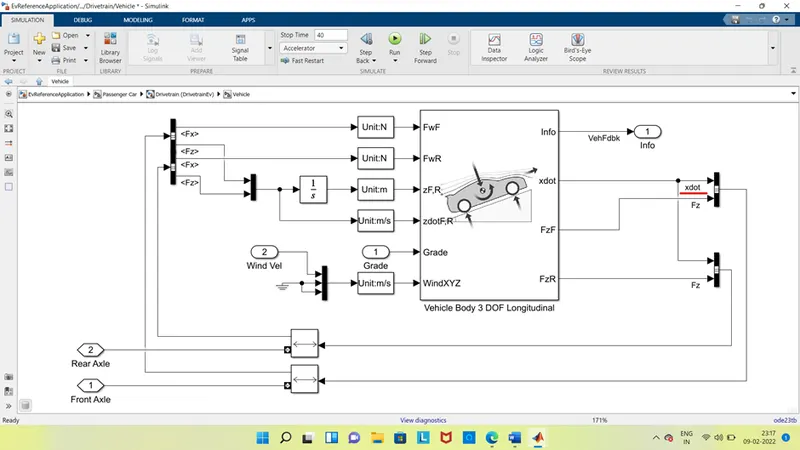
By this Vehicle Body 3 DOF Longitudinal, the output from the xdot block the vehicle speed is being taken.

For the ‘battery power’ block, we can go through ‘EvRefferenceApplication/ Passenger car/ electric plant, as shown.

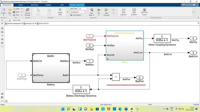
From the above fig at the underlined place, we can get the battery power. It’s a multiplication of battery current and the battery voltage, which is taken from mot current in MotGenEvMapped and battv in battEv, respectively.

On clicking on the EvRefferenceApplication/ visualization we can see the bus selector.

By using the ‘bus selector’ In the visualization all the values are going into it. As shown.

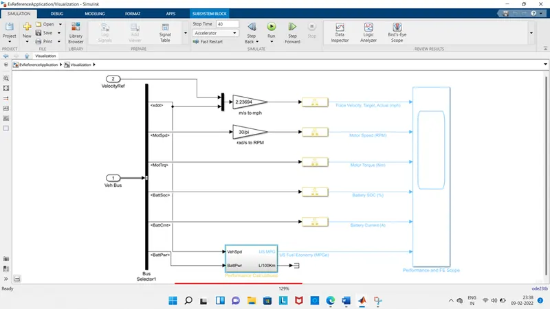
By clicking on the performance characteristics, we can see the calculations of miles per gallon.as shown.

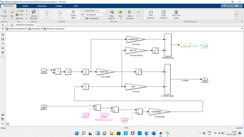
Here first the vehicle speed is converted to meters then to miles in gain block. And

Second the battpwr is converted to kwh to US EPA to s per h to m³ per gal to ramp.

At the end the both are connected to the US MPG CALC product block to get the miles per gallon. In this way the miles per gallon is been calculated.

factors are considered to model fuel flow:

battery power capacity should be high and vehicle power consumption should be low for higher MPGe (miles per gallon equivalent).

vehicle speed.

US EPA equivalent factors can be considered to model fuel flow. That converts the KWH to kwh/USgal.

By changing the value of fuel and fuel capacity, MPGe values can be changed.

3. Run the HEV Reference Application with WOT drive cycle. Change the grade and wind velocity in the environment block. Comment on the results.

Hybrid Electrical Vehicle (HEV):

Hybrid electrical vehicle is a multimode operation vehicle it operates on both electrical motor and mechanical engine that is it’s a combination of an electric propulsion system and conventional internal combustion engine (ICE). This type model vehicles are used for the better fuel economy, than other types of vehicles, high efficiency, better performance, and less losses.

The most common form of HEV is the hybrid electric car, although hybrid electric trucks (pickups and tractors), buses, boats and aircraft also exist.it uses the regenerative breaking which is converted, the vehicles kinetic energy to electrical energy, to store into battery for better performance.

Hybrid Electrical Vehicle multimode reference application:

The hybrid electric vehicle multimode reference application represents a full multimode hybrid electric vehicle (HEV) model with an internal combustion engine, transmission, battery, motor, generator, and associated powertrain control algorithms. Use the reference application for powertrain matching analysis and component selection, control and diagnostic algorithm design, and hardware-in-the-loop (HIL) testing.

The block diagram of Hybrid electrical vehicle is,

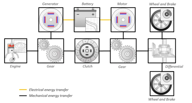
To open the hybrid electric vehicle multimode reference application first go to the ‘getting started with powertrain block set’ through matlab help function, then click on the ‘explore the hybrid electric vehicle multimode reference application’ then we will get the model as below,

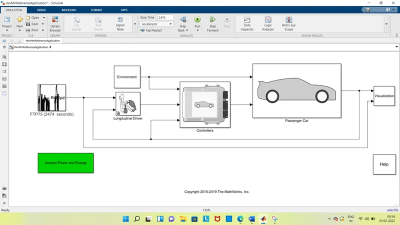
By default, the HEV multimode reference application is configured with:

• Mapped motor and generator.
• 5- l spark- ignition (SI) dynamic engine.
• FTP75 drive cycle with 2474 sec.

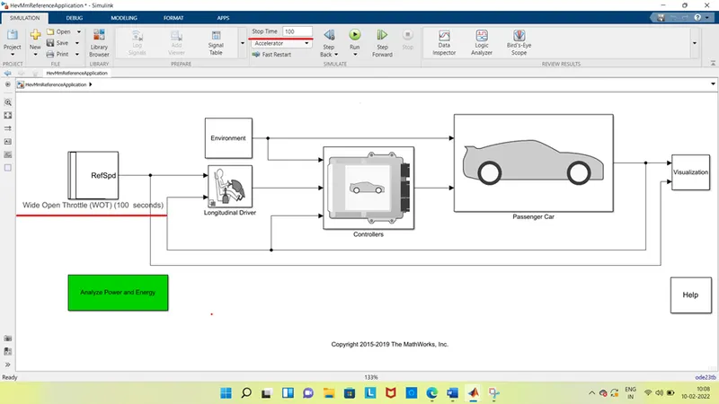
In Hev Mm Reference Application, there are various systems and components like,

Environment, drive cycle, longitudinal driver, passenger car, controllers, visualization.

In this there are various subsystems based on construction.

Based on our condition change the drive cycle from FTP75 to Wide Open Throttle (WOT) with 100 sec.

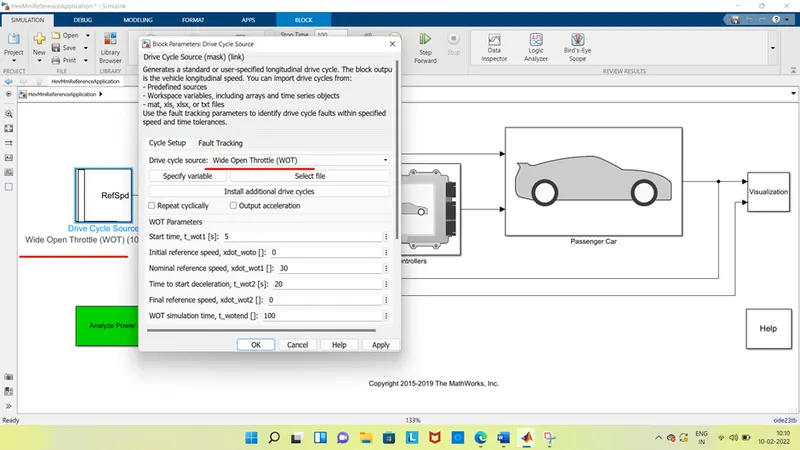
Now run the model with 100 sec stop time as shown.

Results:

The results are optaind in graphical representation in the visualization block in performance and FE scope as shown.

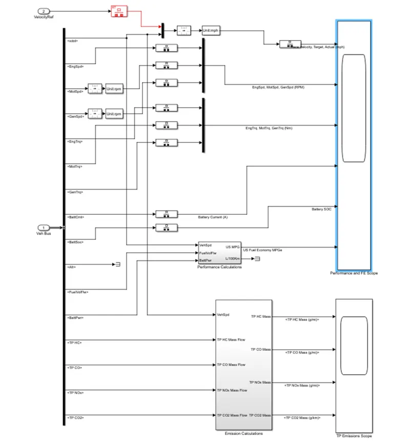
On clicking the scope we will get the graph as shown.

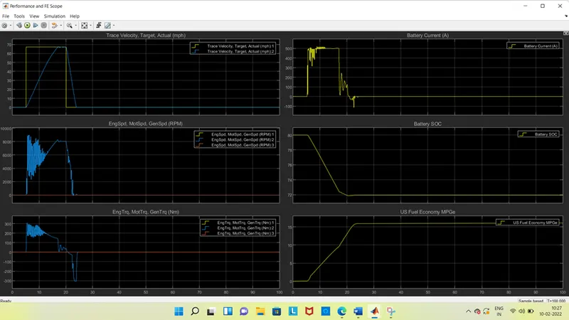
From the results we can say that,

• Trace velocity, target actual (mph) 1 is 0 for 5 sec, because the start time is at 5^th sec and increased from 0 to 67 at 5 sec, and it be constant up to 20 sec, because deceleration time is at 20^th after that it be reduced to 0 up to stop time 100^th sec, because final reference speed is 0.
• Trace velocity, target actual (mph) 2 is also 0 for 5 sec and is increased from 0 to 67.5 as a step type, as a ramp up to 20^th and reduced to 24^th sec after that it be constant up to 100^th sec.
• In the Engspd, Motspd, Genspd (RPM) also starts from 5^th sec and increase up to 8500 rpm, and runs up to 24^th sec with some fluctuations. After it been constant for 100 sec.
• Here also in the EngTrq MoyTrq GenTrq (Nm), its starts from 5^th sec and rages up to 300 nm and reduce to negative path and again gets to 0 at 24^th sec, the changes in the torque are same as the speed values when the speed scope is reduced and the torque is be get to negative side up to 300.
• As we see in the battery current (A) block, it gets activated at the 5^th sec up to 500 A, and it kept constant up to 20^th sec and then try to reduce due to sudden droppage of speed and it goes to negative due to regenerative breaking and been constant at 24^th sec at 0 till 100^th
• As now in the battery soc, the charging capacity is at 80 at starting, whn the vehicle starts running it reduced constantly from 5^th to 24^th sec from 80 to 72.
• As from the US FUEL ECONOMY MPGe it starts from 0 to 16 mpg from 5^th to 24^th sec and runs as constant till 100^th.

HEV model with Change in the grade and wind velocity from the environment block:

Now open the environment subsystem in the HEV reference application.

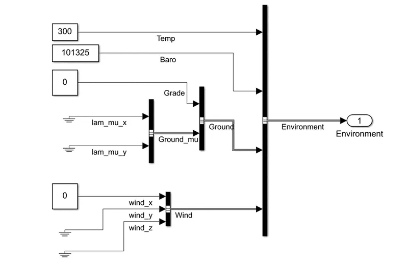
Change the grade value to 10 degrees and wind velocity as 15.

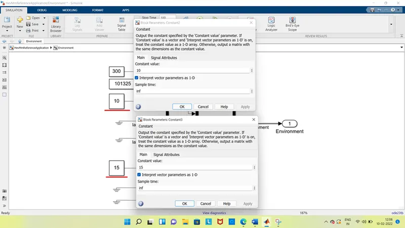
Now run the model for 100 sec and see the results as below.

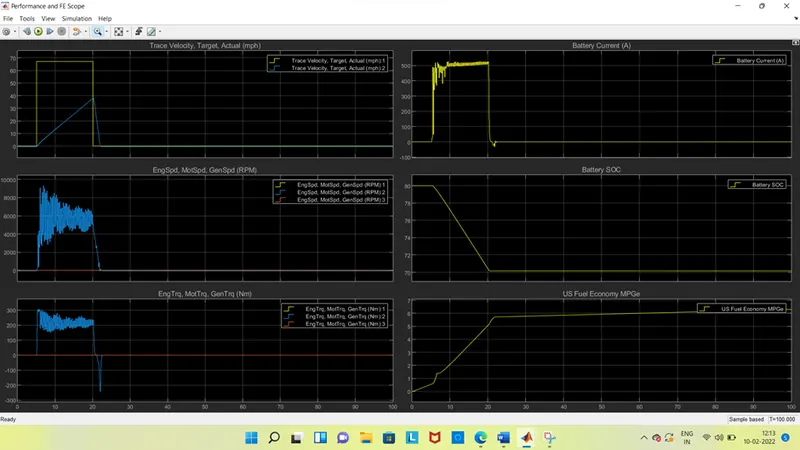
From the results we can say that.

• Trace velocity, target actual (mph) 1 is 0 for 5 sec, and increased from 0 to 67 at 5 sec, and it be constant up to 20 sec, because deceleration time is at 20^th after that it be reduced to 0 up to stop time 100^th sec, because final reference speed is 0.
• Trace velocity, target actual (mph) 2 is also 0 for 5 sec and is increased from 0 to 38 as a step type, as a ramp up to 20^th and reduced to 24^th sec after that it be constant up to 100^th sec.
• In the Engspd, Motspd, Genspd (RPM) also starts from 5^th sec and increase up to 8500 rpm, and runs up to 24^th sec with some fluctuations. After it been constant for 100 sec. the sudden changes as up and down is by change in the wind velocity and grade value.
• Here also in the EngTrq MoyTrq GenTrq (Nm), its starts from 5^th sec and rages up to 300 nm and reduce to negative path and again gets to 0 at 24^th sec, the changes in the torque are same as the speed values when the speed scope is reduced and the torque is be get to negative side up to 300.here also the same fluctuations are repeated as above.
• As we see in the battery current (A) block, there is no changes except at braek time, it gets activated at the 5^th sec up to 500 A, and it kept constant up to 20^th sec and then try to reduce due to sudden droppage of speed and it goes to negative due to regenerative breaking and been constant at 24^th sec as 0 with less dampings till 100^th
• As now in the battery soc, the charging capacity is at 80 at starting, whn the vehicle starts running it reduced constantly from 5^th to 20^th sec from 80 to nearly 70.
• As from the US FUEL ECONOMY MPGe it starts from 0 to 5.7 mpg from 5^th to 22^nd sec and increased constantly runs as constant from 5.7 to 6.3 till 100^th .

1. Keeping all other parameters same, compare the simulated results of hybrid and pure electric powertrains.

EV Reference Application model:

From the ‘getting stared with powertrain block set’ click on the ‘explore the electrical vehicle reference application ‘and we get the model as below.

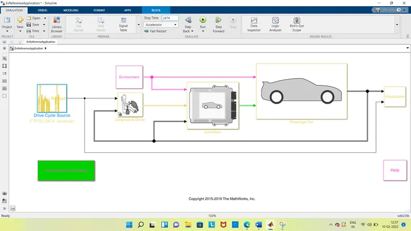
Run the model and see the results in scope by clicking on the visualization and click on the performance and FE scope.

The graphical representation of the scope is shown below.

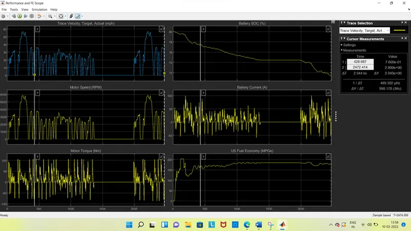
from the results we can say that:

• The trace velocity, target actual (mph) 1, is started at 20 sec, and reaches up to maximum range of 56.5 based on the drive cycle it values are arranged.

It constant at the value from 1360 to 1990

• The trace velocity, target actual (mph) 2 is also same as the trace velocity, target actual (mph) 1 with small changes.
• Motor speed (RPM), when we observe the graph that it is same as that off the trace velocity, target actual (mph) 1 in x axis that is in time in sec, but in the y axis the speed in rpm is rages to 5870.and at the same values the constant range is activate.
• In motor torque (Nm) based on the force applied on the motor for acceleration it plots and it ranges up to 106 from 20^th here also the constant value is been same. Here the damping waves are obtained due to the change in the speed, breaking, acceleration and deceleration.
• When we observe the graph of the battery soc (%) we can say that at starting the battery charging capacity is at 80% after 20 sec when it starts raising the state of charge is being reduced up to 71%. If we observe that at the state of stop time the battery also not in working state, due to off condition.
• When it comes to battery current (A) its look be same as the motor torque, because the current usage is fore=med based on the motor torque, (torque is directly proportional to current).
• If we see the US Fuel Economy (MPGe), at the starting stage it started at 20 sec, and raises up to value of 204 mpge and it raise and fall based on the distance travelled by the vehicle, and it seems be constant when it is in off condition.

HEV Multimode Reference Application model:

From the ‘getting stared with powertrain block set’ click on the ‘explore the hybrid electrical vehicle reference application ‘and we get the model as below.

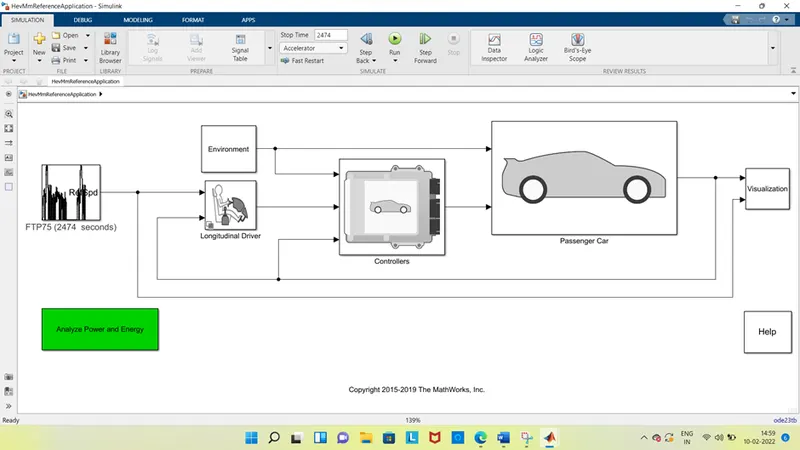
Run the model and see the results in scope by clicking on the visualization and click on the performance and FE scope.

The graphical representation of the scope is shown below.

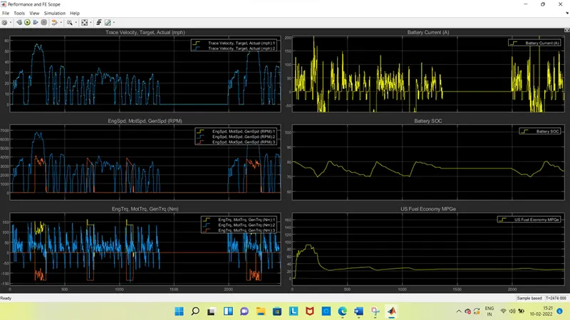
from the results we can say that:

• The trace velocity, target actual (mph) 1, is started at 20 sec, and reaches up to maximum range of 56.5 as same as EV reference application based on the drive cycle it values are arranged.

It constant at the value from 1360 to 1990.

• The trace velocity, target actual (mph) 2 is also same as the trace velocity, target actual (mph) 1 with small changes.
• Motor speed (RPM), when we observe the graph that it is same as that off the trace velocity, target actual (mph) 1 in x axis that is in time in sec, but in the y axis the speed in rpm is rages to 6770.and at the same values the constant range is activate.

Here the RPM 3 has changed the rages due to the engine parameters adding in the model.

• In engine torque, motor torque, generator torque (Nm)1, based on the force applied on the motor for acceleration it plots and it ranges up to 162 from 20^th here also the constant value is been same. Here the damping waves are obtained due to the change in the speed, breaking, acceleration and deceleration.

The engine torque, motor torque, generator torque (Nm)2, reaches max range up to 145 Nm. It places exact same as the same as RPM 3.

The engine torque, motor torque, generator torque (Nm)3, reaches range in negative direction of about 135 Nm, it places same values of the ROM ranges. The changes are observed due to changes in the motor to engine due to get high efficiency.

• When we observe the graph of the battery soc (%) we can say that at starting the battery charging capacity is at 80% after 20 sec when it starts raising the state of charge is being reduced up to 70% in a wave form during the change in the engine and motor based on the working and efficiency. If we observe that at the state of stop time the battery also not in working state, due to off condition. Because of these conditions its flow in charging and discharging because this the battery efficiency increase and used for long time
• When it comes to battery current (A) its look be same as the motor torque, because the current usage is formed based on the motor torque, (torque is directly proportional to current).
• If we see the US Fuel Economy (MPGe), at the starting stage it started at 20 sec, and raises up to value of 90 mpge and it raise and fall based on the distance travelled by the vehicle, and it seems be constant when it is in off condition and small changes in the mpg it been stable at 20 mpge because of the engine usage is started here.

Conclusion:

• Battery current is continuously changing in HEV due to charging and discharging while in pure EV the battery current is continuously discharging.
• The US Fuel Economy is high in EV compared to HEV, travelling cost is less in EV.
• The motor speed (RPM) is high for HEV compared to EV.