Week 7 State of charge estimation

Simulate the 3 test cases from harness dashboard and write a detailed report on the results

Answer:

Simulink model of a BMS close loop harness dashboard:

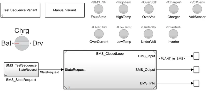
• In the above diagram, the different states of the BMS are given by using the test sequence variant.
• The state request accepts the command and gives it to BMS plant.
• The LEDs are use to indicate the working of the different parts of the system during the simulation.
• The LEDs shows any fault in the system by glowing red.

Simulink model of a BMS close loop system:

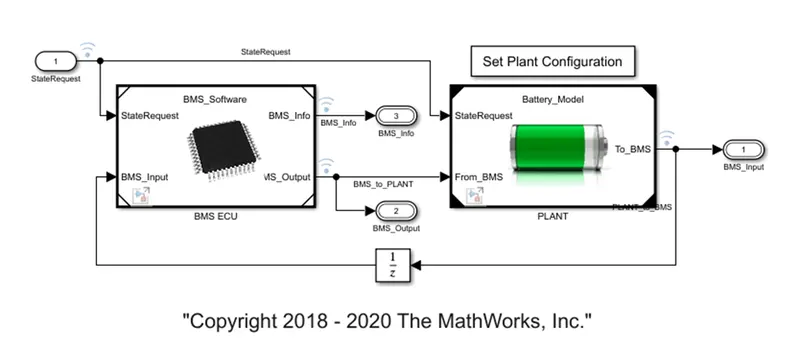
• The BMS is the closed loop system that gives the control signal according to the output requirement.
• The BMS ECU is the electronic control unit which controls the plant by providing necessary signals.
• The ECU implements state machine for logic implementation for different condition, SOC estimation and cell balancing.
• The plant subsystem has motor load and the charger for extra charging.

Test sequence variant 1:

• The test case 1 is choose by selecting 1 number in test sequence variant block as shown in the below diagram.

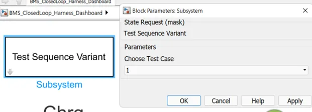
• By selecting 1 number, the command goes to the BMS_StateResponse block for choosing the case 1.
• The test sequence 1 block is activated and it gives the signal of test condition to the BMS electronic control unit.
• The below picture is the block of test sequence which is activated.

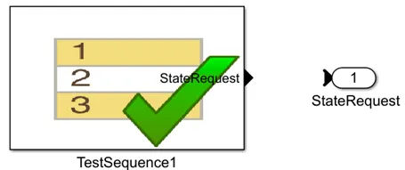
• The test sequence block contains the test conditions of the battery.
• The below picture shows the test conditions.

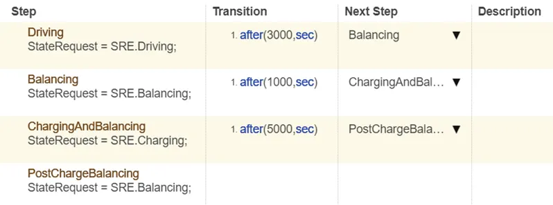
• As seen, there is a driving condition up to 3000 sec.
• During the driving condition, the battery is in the discharging mode.
• After that there is a transition from driving to balancing mode.
• It takes the 1000 sec for the balancing.
• At this point there is a balancing of the battery pack.
• Then the charging of the battery starts from 4000 sec.
• The battery is charging for 5000 sec and after that it is going in the standby mode for rest of the time.

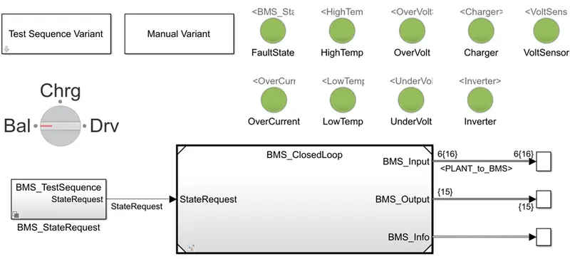
• The above picture shows the dashboard after the completely simulation.
• The test is a smooth, there is no any fault condition.
• So all the LEDS are green in colour.
• The test results are shows in below figure.

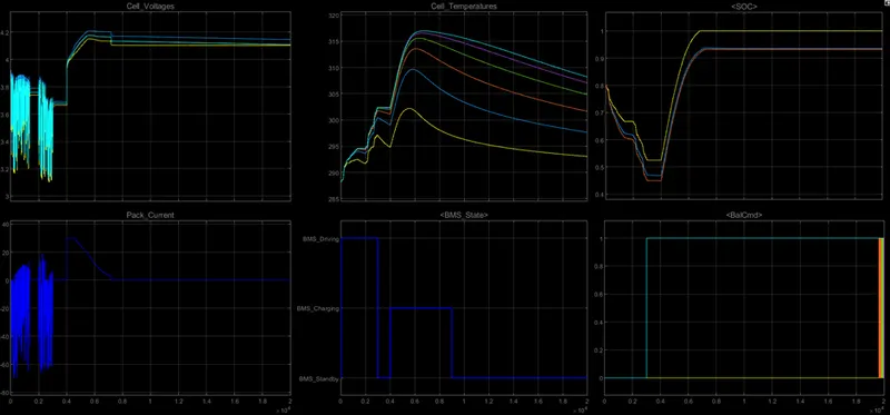
• In the above diagram results for cell voltages, pack current, BMS state, cell temperatures, SOC and balancing commands are shown.
• The first graph is the cell voltages of all the six cells as shown below.

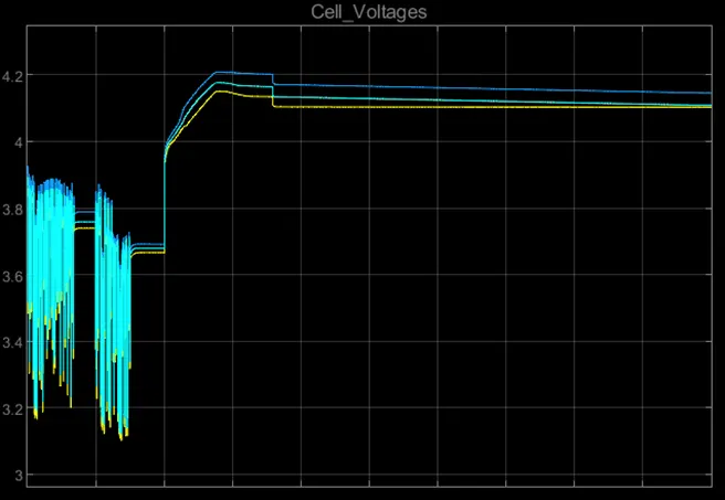
• Initially there is a driving mode up to 3000 sec and cell draws the higher current and voltages.
• Therefore there is a transients up to 3000 sec.
• The transients vary from 3.1 V to 3.9 V.
• After that there is a rest period of the battery for next 1000 sec and voltages are constant at 3.7 V.
• During the charging mode, the voltage rises quickly and comes to the constant voltage value of up to 4.1 V.
• At the end of charging there is a cell balancing occurs and voltages of the cells are balancing with respect to each other.

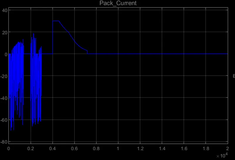
• The picture shows the graph of the battery pack current.
• During the driving condition the battery provides the higher current so there are more fluctuations in the current.
• As the battery is discharging the current is going negative.
• After the battery is at rest for 1000 sec, the current is zero.
• During the charging mode, there is a higher current proving to the battery.
• Therefore the battery current goes high up to 30 A.
• The current is zero during the rest state of the battery.

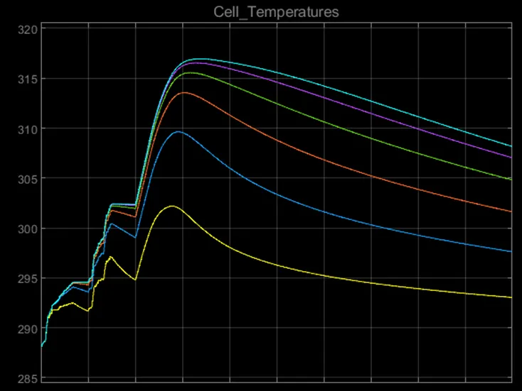
• The above picture shows the temperatures of each cell.
• The temperature of the cell number 6 (blue line) is higher that the cell number 1 (Yellow line).
• The cell number 6 is thermally insulated from one side therefore it is hotter than the cell number 1.
• The temperature of each cell is reducing for some time as there is a standby mode.
• And then increasing during the charging of the battery.
• The graph for each cell is nearly similar in nature.
• This shows that the thermal behaviour of each cell is similar

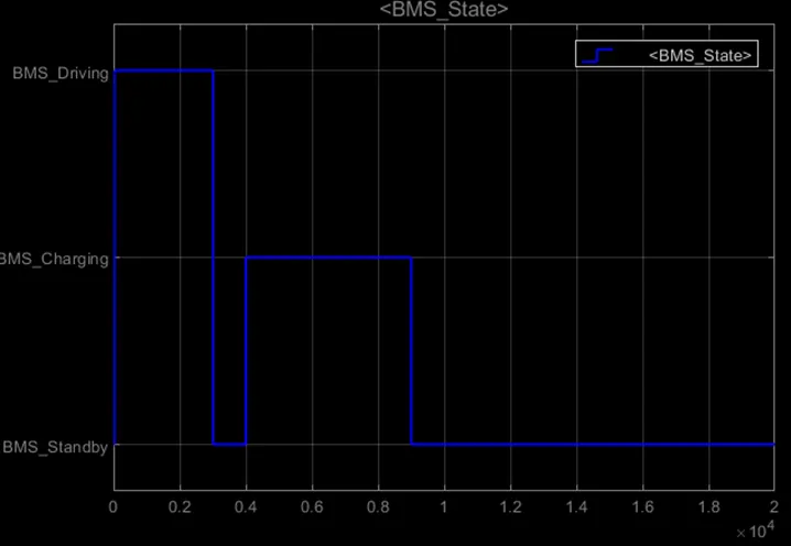
• The above graph shows the BMS state.
• As seen there are three state driving, charging and rest.
• For first 3000 sec, the battery is in drive mode.
• For next 3000 – 4000 sec, the battery module is in the standby mode and balancing each cell.
• From 4000 – 9000 sec the battery is charging and for remaining time the battery module is balancing each cell.

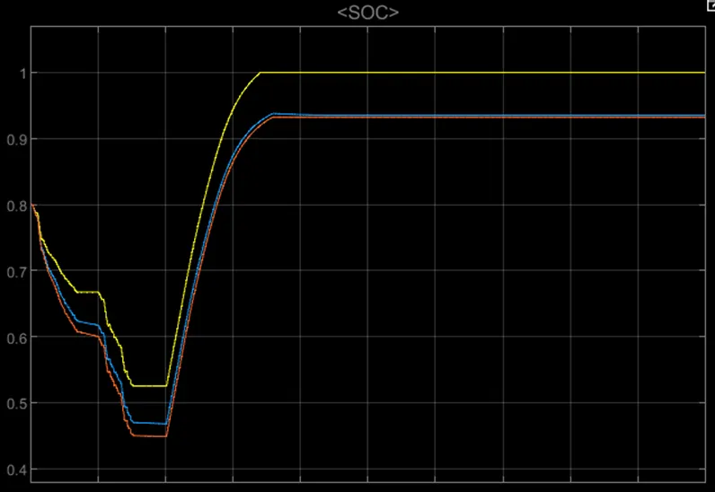
• The above graph shows the SOC estimation for the battery pack which is measured by different technique.
• The yellow line of SOC represents the SOC estimation by the coulomb counting method.
• Blue plot represents the UKF (Unscented Kalman Filter) technique and orange plot represents the EKF (Extended Kalman Filter) technique of SOC estimation.
• The initial SOC of the battery pack is 80 %.
• The SOC is decreases to nearly 45 % during the driving mode.
• It is constant when the battery at rest.
• Then again the SOC is increases as the there is a charging of the battery and at the end of the charging during rest od the battery SOC is constant.
• By Coulombs counting method, the SOC od the battery reaches to 100 %.
• The UKF and EKF method of determining the SOC are nearly the same.

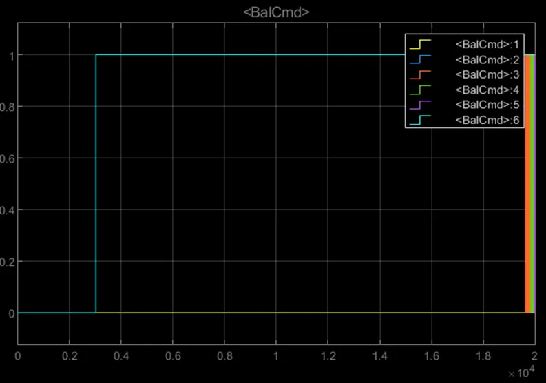
• The graph shows the balancing command for each six cells.
• At the end of the driving state, the balancing is there for 1000 sec.
• It calculates the difference between the higher cell voltage and lower cell voltage.
• At 3000 sec the balancing commands goes to the cell 2 and cell 6 as they have higher voltages during the balancing.
• At this charging and balancing state balancing occurs on cell 2 and cell 6 which remains in state 1 until the end of the simulation.
• The cell 1 representing with the yellow plot remains in the zero state as it has lowest voltage.
• At the end of the simulation each cell try to balance equally so they go into the state 1.

Test sequence variant 2:

• The test case 2 is choose by selecting 2 number in test sequence variant block as shown in the below diagram.

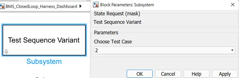
• By selecting 2 number, the command goes to the BMS_StateResponse block for choosing the case 2.
• The test sequence 2 block is activated and it gives the signal of test condition to the BMS electronic control unit.
• The below picture is the block of test sequence which is activated.

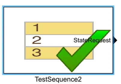
• The test sequence block contains the test conditions of the battery.
• The below picture shows the test conditions.

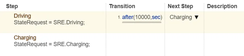
• As seen, there is a driving condition from the start of the simulation.
• During the driving condition, the battery is in the discharging mode.
• The driving condition lasts for 9000 sec.
• After that there is a transition from driving to balancing mode.
• It takes the 1000 sec for the balancing.
• At this point there is a balancing of the battery pack.
• Then the charging of the battery starts from 10,000 sec.

• The above picture shows the dashboard after the completely simulation.
• The test is a smooth, there is no any fault condition.
• So all the LEDS are green in colour.
• The test results are shows in below figure.

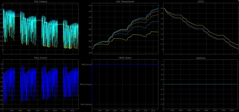
• In the above diagram results for cell voltages, pack current, BMS state, cell temperatures, SOC and balancing commands are shown.
• The first graph is the cell voltages of all the six cells as shown below.

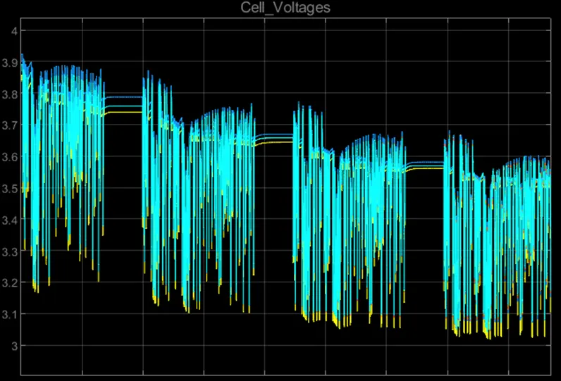
• The cell voltages vary from 3.2 V to 3.9 V at the starting.
• The voltages are reduced at the end of the driving state.
• The voltages drop to 3.05 V to 3.6 V.
• There are more fluctuations in the cell voltages.

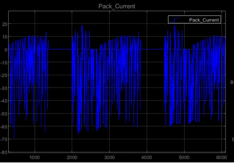
• During the driving condition the battery provides the higher current so there are more fluctuations in the current.
• As the battery is discharging the current is going negative.
• The battery currents drop to 70 A and there are some balancing conditions during the driving mode.
• Sometimes current goes positive due to the charging of the battery.

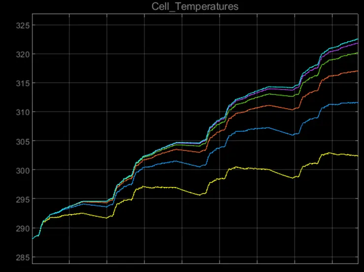
• The above picture shows the temperatures of each cell.
• The temperature of the cell number 6 (blue plot) is higher that the cell number 1 (Yellow plot).
• The cell number 6 is thermally insulated from one side therefore it is hotter than the cell number 1.
• The temperature of each cell is reducing for some time as there is a standby mode in between.
• The graph for each cell is nearly similar in nature.
• This shows that the thermal behaviour of each cell is similar.

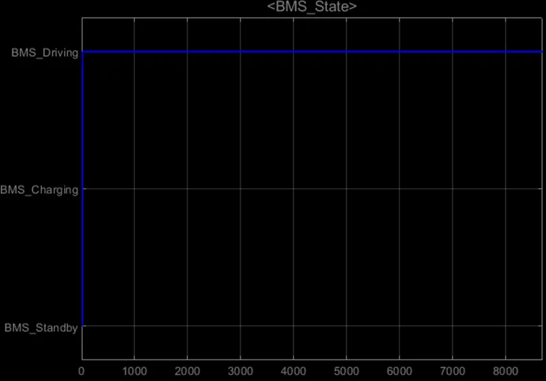
• The above graph shows the BMS state.
• As seen there is only one state as driving.
• There are some stand by modes which are not plotted in the figure.

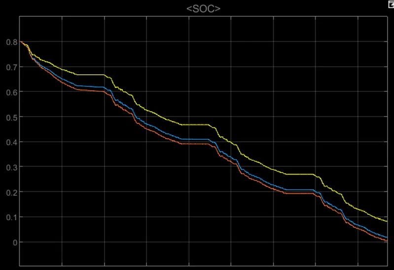
• The above graph shows the SOC estimation for the battery pack which is measured by different technique.
• The yellow line of SOC represents the SOC estimation by the coulomb counting method.
• Blue plot represents the UKF (Unscented Kalman Filter) technique and orange plot represents the EKF (Extended Kalman Filter) technique of SOC estimation.
• The initial SOC of the battery pack is 80 %.
• The battery is dead during the driving mode as SOC reaches to 0.
• The UKF and EKF method of determining the SOC are nearly the same.
• The nature of graph for SOC estimation for all three techniques are nearly same.

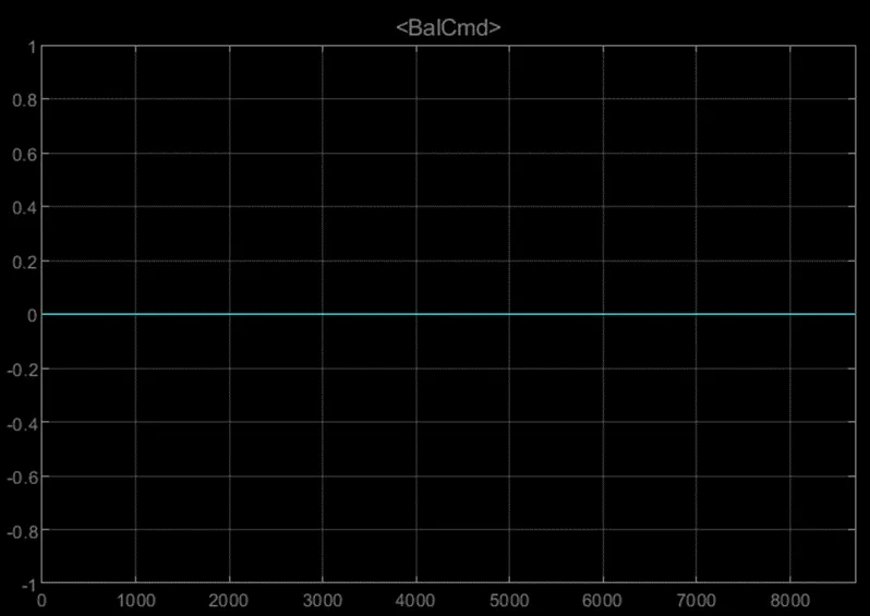
• Here the cells are balanced for entire driving condition.

Test sequence variant 3:

• The test case 3 is choose by selecting 3 number in test sequence variant block as shown in the below diagram.

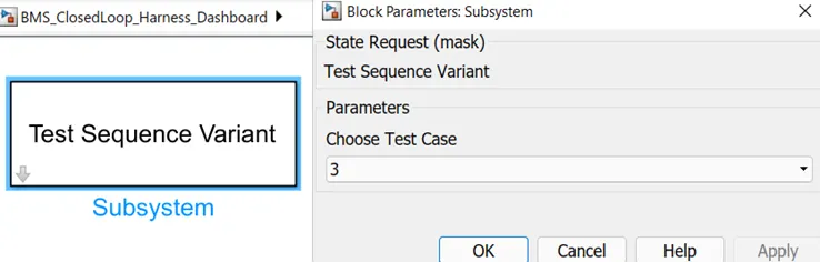
• By selecting 3 number, the command goes to the BMS_StateResponse block for choosing the case 3.
• The test sequence 3 block is activated and it gives the signal of test condition to the BMS electronic control unit.
• The below picture is the block of test sequence which is activated.

• The test sequence block contains the test conditions of the battery.
• The below picture shows the test conditions.

• As seen, there is a charging condition from the start of the simulation.
• The battery is fully charged up to 2000 sec and then there is a balancing of the cell throughout simulation.

• The above picture shows the dashboard after the completely simulation.
• The test is a smooth, there is no any fault condition.
• So all the LEDS are green in colour.
• The test results are shows in below figure.

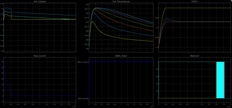
• In the above diagram results for cell voltages, pack current, BMS state, cell temperatures, SOC and balancing commands are shown.
• The first graph is the cell voltages of all the six cells as shown below.

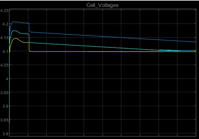
• The cell voltages vary from 4.1 V to 4.2 V at the starting.
• At 2000 sec the battery is completely charged and voltages are constant at 4.1 V.
• There is a balancing of the voltages after the 2000 sec.

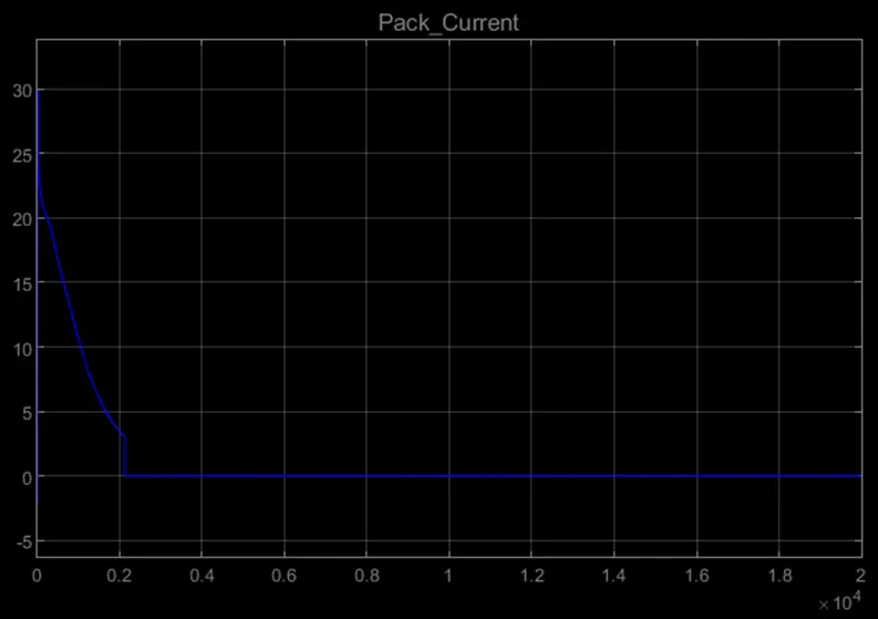
• During the charging condition the current is provided to the battery.
• The initial rise of current is up to 30 A.
• After the complete charging of the battery, the current supplied is zero.

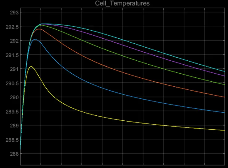
• The above picture shows the temperatures of each cell.
• The temperature of the cell number 6 (blue plot) is higher that the cell number 1 (Yellow plot).
• The cell number 6 is thermally insulated from one side therefore it is hotter than the cell number 1.
• The temperature of all cells is increasing in the charging mode.
• After the charging the temperatures are decreasing due to the balancing of the cells.
• The graph for each cell is nearly similar in nature.
• This shows that the thermal behaviour of each cell is similar.

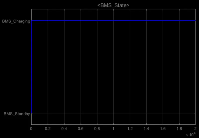
• The above graph shows the BMS state.
• As seen, there is only one state as charging.

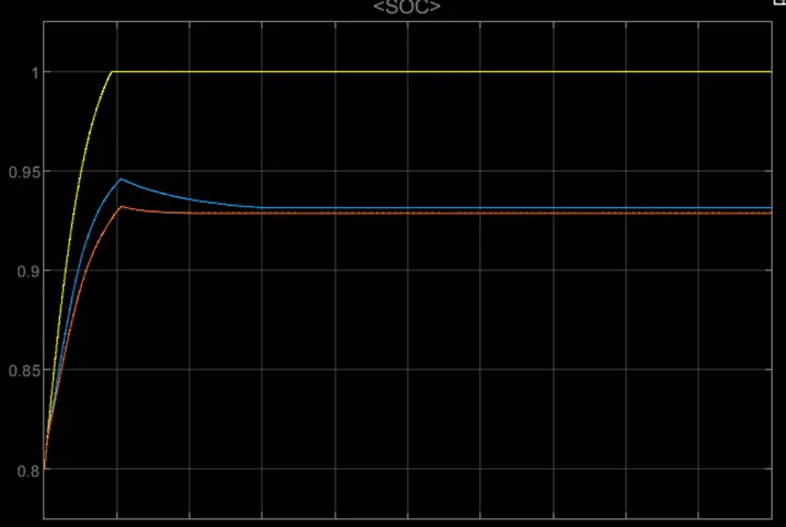
• The above graph shows the SOC estimation for the battery pack which is measured by different technique.
• The yellow line of SOC represents the SOC estimation by the coulomb counting method.
• Blue plot represents the UKF (Unscented Kalman Filter) technique and orange plot represents the EKF (Extended Kalman Filter) technique of SOC estimation.
• The initial SOC of the battery pack is 80 %.
• The SOC of the battery is increasing due to the charging.
• The battery is fully charged at 2000 sec.
• The SOC estimation by the Coulomb counting method is reaching the 100 % value at 2000 sec.
• The UKF and EKF method of determining the SOC are nearly the same and reaches to the 93 % during the simulation.
• The nature of graph for SOC estimation for all three techniques are nearly same.

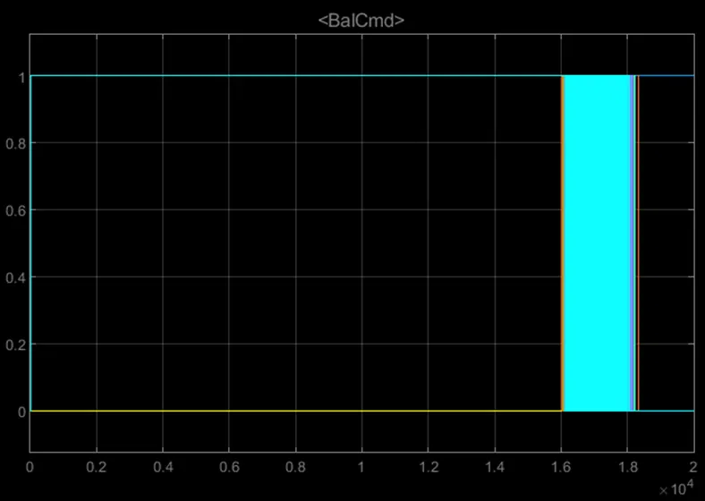
• The graph shows the balancing command for each six cells.
• At the starting of the simulation the voltages of the cells 2 and 6 are higher so they go into the balancing mode as state 1.
• At the end of the simulation each cell tries to balance equally so they go into the state 1.
• At the end the voltage of the cell 2 is still higher so it remain in the state 1.

Coulomb counting:

The coulomb counting methods measures the SOC of the battery at the end of the charging and the discharging of the battery. It measures the charging and the discharging current of the battery and integrated it with respect to time to calculate SOC.

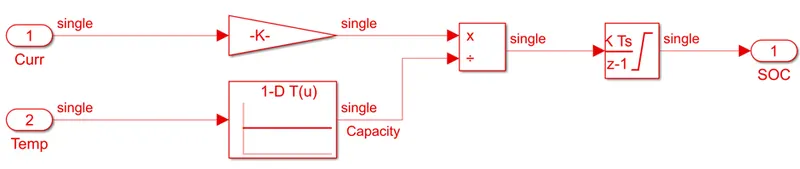
• The below figure shows the SOC calculation in the BMS close loop model.
• The SOC is calculated by using the battery pack current and the temperature of the cell number six as shown in below figure.

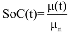
• The formula to calculate the SOC is given below:

Where,

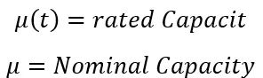
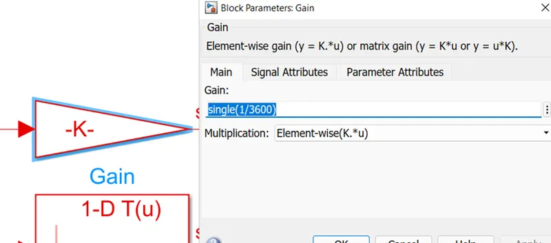
• The current of the battery pack is divided by the 3600 sec to convert it into Ahr capacity which is the rated capacity of the battery.
• The figure below shows the gain value of 1/3600 which is multiply by current.

• The temperature of the cell number 6 is taken for the nominal capacity calculation of the battery as it is having the highest temperature of all.
• The temperature is given to the lookup table which converts it into the nominal capacity.
• According to the formula given above rated capacity of the battery is divided by the nominal capacity and integrated it with respect to the time which gives the SOC of the battery.