Week 7 - Simulation of a 1D Supersonic nozzle flow simulation using Macormack Method

Question :

In this challenge you are going to simulate the isentropic flow through a quasi 1D subsonic-supersonic nozzle. You will derive both the conservation and non-conservation forms of the governing equations and sovle them using the MacCormack's technique. You need to determine the steady-state temperature distribution for the flow-field variables and investigate the difference between the two forms of governing equations by comparing their solutions.

You need to show the following plots inside your report
1. Steady-state distribution of primitive variables inside the nozzle
2. Time-wise variation of the primitive variables
3. Variation of Mass flow rate distribution inside the nozzle at different time steps during the time-marching process
4. Comparison of Normalized mass flow rate distributions of both forms

Expected Results:

• Perform a grid independence test on the solution and expain all your findings.
• The code must be modular. You need to write separate functions to solve both forms.
• Discuss all the plots you are providing with observed inferences.  

Explanation :

Mach number

The Mach number,often denoted as 'ma' is a dimensionless quantity that represents the speed of an objest or fluid relative to speed of sound in that medium. The mach usmber is calculated using the formula:

Mach number(ma) = (Speed of Object/fluid(v))/ Speed of sound in medium(c)

In this formula(ma): The speed of the object or fluid (v) is the velocity of the object or fluid in meter per second(m/s)or any other appropriate unit of speed.

The speed of sound in medium (c) is the velocity at which pressure waves, or sound waves, propagate through that specific medium, such as air, water or a solid material. The speed of sound varries depending on the medium properties, such as temp and perssure. 

The mach no is used extensively in aerodynamics and fluid dynamices to describe the behavior of objects, such as aircraft,missiles or projectiles as thet move through a fluid. It categorizes the object's speed into different regimes:

Ma<1>

Ma = 1: Transonic flow - The object is travling at a speed of sound, often associated with the onest of compressibility effects.

Ma>> 1: Hypersonic flow - The object is traveling at an extemely high speed relative to the speed of sound, often reqiring specialied aerodynamic considerations.

MacCormack method :

The MacComack method,also known as the Maccormak predictor-Corrector method,is a numerical techique used for solving partial differential equations(PDEs), particularly in the field of CFD. It is an explicit finite-difference method commonly used for simulating the time evolution of fluid flow problems.

The maccormack method is a two step process that combines a predictor step with a corrector step to approximate the solution to PDe. Here's a brief overview of how the method works:

Predictor Steps:

In the predictor step, an initial approximatetion for the solution is calculated using a forward time-stepping scheme.The step is often referred to as the "predictor" because it provides an estimate of the solution at the next time level.

It typically involves a finite-difference scheme,such as the "predictor" because it provides an estimate of the solution at the next time level.

It typically involves a finite-difference scheme,such as the forward Euer method,to update the solution from the current time level to a ' predicted' time level.

Corrector Step:

In the corrector step,the predictor step's result is used to improve the accuracy of the solution.The step is often referred to as the 'corrector' because it corrects the prediction made in the previous step.

It involves another finnite-difference scheme,usually a backward time-stepping scheme,to compute corrections to the predicted values.These corrections are then added to predictor's results to obtain a more accurate solution at the next time level.

The maccormack method is particularly used for solving time-dependent PDEs,including the Euler equations and the Navier-Stokes eqn,which describe fluid flow.It is a stable and staightforward approach for simulating fluid dynamics and other physical phemomena, especially in cases where high accuracy is not required.

Continuity equation :

 In fluid dynamics, the continuity equation is a fundamental equation that describes the conservation of mass within a fluid flow. It is expressed mathematically as:

Where:

• `(deltarho)/(deltat)`​ represents the rate of change of density (`delta`ρ) with respect to time (`delta`t).
• `delta(rho v)` represents the divergence of the mass flux, where `delta`ρ is the density and `delta`v is the velocity vector.

In one-dimensional form (along a single spatial coordinate x), the continuity equation becomes:

This equation states that the change in density with respect to time is equal to the negative divergence of the mass flux (ρv) along the x direction.

Momentum equation: 

In the conservative form, the momentum equation is written as follows for a one-dimensional case along the x-direction:

`delta/(deltat)(rho*u*A)+delta/(deltax)(rho*u^2*A) = rho y A -delta/(deltax)(rho*A)`

Where:

• ρ is the density of the fluid.
• u is the velocity in the x-direction.
• A is the cross-sectional area of the nozzle.
• P is the pressure.
• g is the acceleration due to gravity.

Energy equation : 

In a general form, the one-dimensional energy equation for a compressible fluid flow along the x-direction can be written as:

Where:

• `rho` is the density of the fluid.
• E is the total energy per unit mass (internal energy + kinetic energy).
• A is the cross-sectional area of the flow.
• u is the velocity in the x-direction.
• h is the specific enthalpy.
• T is the temperature.
• k is the thermal conductivity.
• P is the pressure.
• `g_x`​ is the acceleration due to gravity in the x-direction.

The terms in the equation represent various contributions to energy conservation, including changes in internal energy, kinetic energy, heat conduction, work done by pressure forces, and work done by gravitational forces.

 We use the equations in this form :

Answer :

Main code:

clear all
close all
clc
%input
n = 31 ;
x = linspace(0,3,n);
dx = x(2) - x(1);
gamma = 1.4;
%time steps
nt = 1400;
c = 0.5;
throat=((n+1)/2);
 
 
%area
a = 1+2.2*(x-1.5).^2;
 
 
 
 
[v,rho,t,mach_number,mass_flow_rate,pressure,dt,rho_t,v_t,t_t,pressure_t,mach_number_t]=non_conservative_week_seven(x,gamma,dx,a,n,nt,c,throat)
 
[Vc,rhoc,tc,cons_mass_flow_throat,Mc,pc,Vc_throat,rho_throat,T_throat,cons_mass_flow,Mc_throat,pc_throat]=conservative_week_seven(throat,x,gamma,dx,a,n,nt,c)
 
figure(2)
plot(x,rho,'linewidth',1.5)
hold on
plot(x,rhoc,'linewidth',2.5)
xlabel('distance of nozzle(x)');
ylabel('density');
legend('non conservative form','conservative form');
title('density profile');
grid on
 
figure(3)
plot(x,t,'linewidth',1.5);
hold on
plot(x,tc,'linewidth',1.5)
xlabel('distance of nozzle(x) ');
ylabel('Temperature');
legend('non conservative form','conservative form');
title('Temperature change');
grid on
 
figure(4)
 
plot(x,mach_number,'linewidth',1.5);
hold on
plot(x,Mc,'LineWidth',1.5)
xlabel('distance of nozzle(x) ');
ylabel('Temperature');
legend('non conservative form','conservative form');
title('mach_number');
grid on
 
 
figure(5)
plot(x,v,'linewidth',1.0);
hold on
plot(x,Vc)
xlabel('distance of nozzle(x)');
ylabel('velocity');
legend('non conservative form','conservative form');
title('Velocity profile');
grid on
 
figure(6)
plot(x,pressure,'linewidth',1.0);
hold on
plot(x,pc,'linewidth',1.5)
xlabel('distance of nozzle(x)');
ylabel('velocity');
legend('non conservative form','conservative form');
title('pressure');
grid on
 
 
figure(7)
plot(x,mass_flow_rate,'linewidth',1.0);
hold on
plot(x,cons_mass_flow);
xlabel('distance of nozzle(x)');
ylabel('velocity');
legend('non conservative form','conservative form');
title('mass_flow_rate');
grid on
 
figure(8)
plot(rho_t)
hold on
plot(T_throat)
legend('non conservative')
xlabel('time step')
ylabel('density')
title('rho at throtal')
grid on
 
figure(9)
plot(mach_number_t)
hold on
plot(Mc_throat)
xlabel('time step')
ylabel('mach number')
legend('non conservative')
title('temp at trotal')
grid on
 
figure(10)
plot(pressure_t)
hold on
plot(pc_throat)
xlabel('time step')
ylabel('pressure')
legend('non conservative')
title('pressure at trotal')
grid on
 
figure(11)
plot(v_t)
hold on
plot(Vc_throat)
xlabel('time step')
ylabel('velocity')
legend('non conservative')
title('velocity at trotal')
grid on

 

 Explanation of main code :

 

Setting up parameters:

• "n" is the number of spatial grid points. In this case there are 31 grid points.
• "x" is an array of spatial coordinaes ranging from 0 to 3, divided into n evenly spaced points.These points represent positions along the nozzle.
• "dx" is the spatial grid spacing , calculated as the difference between adjacent elements of x.
• "gamma" is the spatial grid spacing, calculated as the difference between adjacent elements of x.
• "nt" is the number of time steps for the simulation,set to 1400.
• "c" is a constant.
• "throat" is caculated as the position of nozzle throat,which is assumed to be at the midpoint of spatial grid.

Defining Nozzle area profile:

 

'a' is an array representing the cross sectional area profile of nozzle. The nozzle geomatry is defined by this profile,and it varies with spatial coordinates x.

 Caling functions : 

The code calls two seprate functions , n non_conservative_week_seven and Conservative_week_seven,which presumable perform calculations replated to fluid slow in a converging - diverging nozzle. These functions accept various inputs and return multiple flow properties at different spatial and temporal points within the nozzle.

 

Plotting Result :

The code creates several figures to visualize the simulation results. Here's a breakdown of each figure:

FIgure 2 to 7: These fiures compare various flow properties(density,temprature,Mach no,velocity,pressure,mass flow rate) between two diffrent forms of governing equations : the non- conservative form and the conservative form and the conservative form. These companisons are made along the spatial coordinates xwithin nozzle.

Figure 8 to 11 : These figures show the evolution of specific flow proerties (density,Mach number,pressure,velocity)at the nozzle throat(throttal)over the course of multiple time steps for the non-conservative and conservative forms.

 

Legend and Labels :

Each figure is weel-labeled with apropriate axes labels and titles for clarity.Legends are also included to distinguish between results obtained using the non- conservative and conservative forms of eqations.

Grid on :

The grid on command is used to overlay a grid on each plot to aid in visual interpretaion.

 

 

 

conservatie :

 

 

%conservative form
function [Vc,rhoc,Tc,cons_mass_flow_throat,Mc,pc,Vc_throat,rho_throat,T_throat,cons_mass_flow,Mc_throat,pc_throat]=conservative_week_seven(throat,x,gamma,dx,A,n,nt,C)
 
R=8.314;
for i=1:n
if (x(i)<=0.5)
rho_in (i)=1;
T_in(i)=1;
elseif (x(i)>=0.5) && (x(i) <= 1.5)
rho_in(i)=1-(0.366*(x(i)-0.5));
T_in(i)=1-0.167*(x(i)-0.5);
else
rho_in(i)=0.634-0.3879*(x(i)-1.5);
T_in(i)=0.833-0.3507*(x(i)-1.5);
end
end
 
u_in=0.59./(rho_in.*A);
rhoc = rho_in;
Tc=T_in;
Vc=u_in;
 
 
 
 
 
dt=0.0206;
t_sim=(nt-1)*dt;
t=0:dt:t_sim;
 
U1=rhoc.*A;
U2=rhoc.*A.*Vc;
U3=rhoc.*A.*((Tc/(gamma-1))+(0.5*gamma.*Vc.*Vc));
 
%Macormack method
for j=1:length(t)
U1_old=U1;
U2_old=U2;
U3_old=U3;
 
F1=U2;
F2=((U2.^2)./U1)+((gamma-1)/gamma).*(U3-((gamma/2)*(U2.^2./U1)));
F3=((gamma.*U2.*U3)./U1)-((gamma*(gamma-1))/2)*(U2.^3)./(U1.^2);
 
%predictor method
for k=2:n-1
dA_dx(j)=(A(k+1)-A(k))/dx;
dlogA_dx = (log(A(k+1))-log(A(k)))/dx;
J2(k)=dlogA_dx*((gamma-1)/gamma)*(U3(k)-(0.5*gamma*U2(k)^2)/(U1(k)));
 
 
%continuity step
 
dF1_dx_p=(F1(k+1)-F1(k))/dx;
dU1_dt_p(k)=-dF1_dx_p;
%momentum equation
dF2_dx_p=(F2(k+1)-F2(k))/dx;
dU2_dt_p(k)=-dF2_dx_p+J2(k);
 
dF3_dx_p=(F3(k+1)-F3(k))/dx;
dU3_dt_p(k)=-dF3_dx_p;
 
U1(k)=(dU1_dt_p(k).*dt)+U1_old(k);
U2(k)=(dU2_dt_p(k).*dt)+U2_old(k);
U3(k) = (dU3_dt_p(k).*dt)+U3_old(k);
end
%applying boundry condition
%input
U1(1)=A(1);
U2(1)=2*U2(2)-U2(3);
U3(1)=U1(1)*((Tc(1)/(gamma-1)+((gamma/2)*Vc(1)^2)));
%output
U1(n)=2*U1(n-1)-U1(n-2);
U2(n)=2*U2(n-1)-U2(n-2);
U3(n)=2*U3(n-1)-U3(n-2);
 
rhoc=U1./A;
Tc=(gamma-1).*((U3./U1)-((gamma/2).*(U2./U1).^2));
 
F1=U2;
F2=((U2.^2)./U1)+((gamma-1)/gamma).*(U3-((gamma/2)*(U2.^2./U1)));
F3=((gamma.*U2.*U3)./U1)-((gamma*(gamma-1))/2)*(U2.^3)./(U1.^2);
 
%corrector method
for k=2:n-1
dA_dx(j)=(A(k)-A(k-1))/dx;
dlogA_dx=(log(A(k))-log(A(k-1)))/dx;
J2(k)=dlogA_dx*((gamma-1)/gamma)*(U3(k)-(0.5*gamma*U2(k)^2)/(U1(k)));
 
%continuity step
dF1_dx_c=(F1(k)-F1(k-1))/dx;
dU1_dt_c(k)=-dF1_dx_c;
 
%momentum equation
dF2_dx_c=(F2(k)-F2(k-1))/dx;
dU2_dt_c(k)=-dF2_dx_c +J2(k);
 
%energy equation
dF3_dx_c=(F3(k)-F3(k-1))/dx;
dU3_dt_c(k)=-dF3_dx_c;
end
for pc=2:n-1
dU1_dt_avg(pc)=0.5*(dU1_dt_c(pc)+dU1_dt_p(pc));
dU2_dt_avg(pc)=0.5*(dU2_dt_c(pc)+dU2_dt_p(pc));
dU3_dt_avg(pc)=0.5*(dU3_dt_c(pc)+dU3_dt_p(pc));
 
U1(pc)=(dU1_dt_avg(pc)*dt)+U1_old(pc);
U2(pc)=(dU2_dt_avg(pc)*dt)+U2_old(pc);
U3(pc)=(dU3_dt_avg(pc)*dt)+U3_old(pc);
end
 
%boundry
%input
U1(1)=A(1);
U2(1)=2*U2(2)-U2(3);
U3(1)=U1(1)*((Tc(1)/(gamma-1)+((gamma/2)*Vc(1)^2)));
%input
U1(n)=2*U1(n-1)-U1(n-2);
U2(n)=2*U2(n-1)-U2(n-2);
U3(n)=2*U3(n-1)-U3(n-2);
 
 
rhoc=U1./A;
Vc=U2./U1;
Tc=(gamma-1)*((U3./U1)-((gamma/2).*(Vc.^2)));
 
pc=rhoc.*Tc;
Mc=Vc./(Tc.^0.5);
cons_mass_flow=rhoc.*Vc.*A;
%variables at throat
rho_throat(j)=rhoc(throat);
T_throat(j)=Tc(throat);
pc_throat(j)=pc(throat);
Mc_throat(j)=Mc(throat);
cons_mass_flow_throat(j)=cons_mass_flow(throat);
Vc_throat(j)=Vc(throat);
 
figure(12)
if j==50
plot(x,cons_mass_flow,'b','linewidth',1.5);
hold on
elseif j==100
plot(x,cons_mass_flow,'r','linewidth',1.5)
hold on
elseif j==150
plot(x,cons_mass_flow,'c','linewidth',1.5)
hold on
elseif j==300
plot(x,cons_mass_flow,'g','linewidth',1.5)
hold on
elseif j==600
plot(x,cons_mass_flow,'y','linewidth',1.5)
hold on
elseif j==900
plot(x,cons_mass_flow,'*','linewidth',1.5)
hold on
elseif j==1400
plot(x,cons_mass_flow,'m','linewidth',1.5)
hold on
 
 
end
end
xlabel('Non dimensioanl distance through nozzle(x)','fontsize',10)
ylabel('Non dimensional mass flow rate through nozzle x','fontsize',10);
title('variation of mass flow rate (conservation form) along x at different time steps');
legend({'50 time steps','100 time steps','150 time steps','300 time steps','600 time steps','900 time steps','1400 time steps'});
end​

 

 

 

Explanation of conservative 

Input Parameters:

• throat: This variable is used to specify the location of the nozzle throat, which was previously calculated as the midpoint of the spatial grid.
• x : An array representing the spatial coordinates within the nozzle.
• gamma: The specific heat ratio of the fluid.
• dx: The spatial grid spacing.
• A : An array representing the cross-sectional area profile of the nozzle, which varies with spatial coordinates x.
• n: The number of spatial grid points.
• nt: The number of time steps for the simulation.
• C: A constant.

Initialization:

• The function starts by defining physical properties (density and temperature) at different spatial locations within the nozzle based on the spatial coordinate x. These initial conditions are defined in regions with x values less than 0.5, between 0.5 and 1.5, and greater than 1.5.
• Initial velocity u_in is calculated based on the initial density and area profile.
• The conservative variables rhoc, Tc, and Vc are initialized with the initial conditions.

Time Integration:

• The simulation is performed over multiple time steps (nt) with a time step size of dt. It initializes a time array t.
• The conservative variables u1, u2, and u3 are initialized based on the initial conditions and are used to represent the conservative form of the flow variables (mass, momentum, and energy) at each spatial point.

MacCormack Method:

• The code then enters a loop over time steps.
• Inside the loop, it calculates the fluxes F1, F2, and F3 based on the current conservative variables.
• The predictor step updates the conservative variables (U1, U2, and U3) using finite differences and the fluxes.
• Boundary conditions are applied for the inlet and outlet.

Corrector Method:

• The code enters another loop to perform the corrector step.
• It calculates the fluxes and updates the conservative variables using an average of the predictor and corrector values.

Boundary Conditions:

• Boundary conditions are applied for both the inlet and outlet to maintain stability and continuity of the simulation.

Calculations and Results:

• After the time integration loops, the code calculates various flow properties like density (rhoc), temperature (Tc), velocity (Vc), pressure (pc), Mach number (Mc), and mass flow rate (cons_mass_flow_rate) based on the conservative variables.
• The variables at the throat of the nozzle are also extracted and stored for analysis.

Visualization:

• The code includes code for plotting the variation of mass flow rate along the nozzle at different time steps (figure(12)). It plots the mass flow rate profile at different stages of the simulation.

Legend and Labels:

• Appropriate labels and legends are added to the plot to provide clarity.

 

 non conservative

 

CODE :

 

 

function [v,rho,t,mach_number,mass_flow_rate,pressure,dt,rho_t,v_t,t_t,pressure_t,mach_number_t]=non_conservative_week_seven(x,gamma,dx,a,n,nt,c,throat);
 
 
calculate initial profile
rho = 1-0.3146*x;
t = 1-0.2314*x;
v = (0.1+1.09*x).*t.^0.5;
 
for n = 1:31
dt_new(n) = (c.*(dx/(a(n)+v(n))));
end
dt = max(dt_new)
 
 
for k = 1:nt
rho_old = rho;
v_old = v;
t_old = t;
 
%pridicted method
for j = 2:n-1
dvdx(j) = (v(j+1)-v(j))/dx;
dlogdx(j) = (log(a(j+1))-log(a(j)))/dx;
drhodx(j) = (rho(j+1) - rho(j))/dx;
dtdx(j) = (t(j+1)-t(j))/dx;
 
%continuty eqn
drho_dt_p(j) = -rho(j)*dvdx(j)-(rho(j)*v(j)*dlogdx(j))-(v(j)*drhodx(j));
 
%momentum eqn
dvdt_p(j) = -(v(j)*dvdx(j)) - (1/gamma)*(dtdx(j) + (t(j)/rho(j))*drhodx(j));
 
%energy
dtdt_p(j) = -(v(j)*dtdx(j)) - ((gamma-1)*t(j)*(dvdx(j) + (v(j)*dlogdx(j))));
 
%solution update
v(j) = v(j) +dvdt_p(j)*dt;
rho(j) = rho(j)+ drho_dt_p(j)*dt;
t(j) = t(j)+ dtdt_p(j)*dt;
 
 
 
end
 
 
 
% corrected method
for j = 2:n-1
dvdx(j) = (v(j)-v(j-1))/dx;
dlogdx(j) = (log(a(j))-log(a(j-1)))/dx;
drhodx(j) = (rho(j) - rho(j-1))/dx;
dtdx(j) = (t(j)-t(j-1))/dx;
 
%continuty eqn
drho_dt_c(j) = -(rho(j)*dvdx(j))-(rho(j)*v(j)*dlogdx(j))-(v(j)*drhodx(j));
 
%momentum eqn
dvdt_c(j) = -(v(j)*dvdx(j)) - (1/gamma)*(dtdx(j) + (t(j)/rho(j))*drhodx(j));
 
%energy
dtdt_c(j) = -(v(j)*dtdx(j)) - (gamma-1)*t(j)*(dvdx(j) + v(j)*dlogdx(j));
 
 
%average of derivative
drhodt(j) = 0.5*(drho_dt_c(j)+drho_dt_p(j));
dvdt(j) = 0.5*(dvdt_p(j)+dvdt_c(j));
dtdt(j) = 0.5*(dtdt_c(j)+dtdt_p(j));
 
end
 
%final solution update
for i = 2:n-1
rho(i) = rho_old(i)+drhodt(i)*dt;
v(i) = v_old(i)+dvdt(i)*dt;
t(i) = t_old(i)+dtdt(i)*dt;
end
 
%boundary condition
%inlet
v(1) = 2*v(2) - v(3);
%outlet
v(n) = 2*v(n-1) - v(n-2);
rho(n) = 2*rho(n-1) - rho(n-2);
t(n) = 2*t(n-1) - t(n-2);
 
 
 
mass_flow_rate = rho.*a.*v;
pressure = rho.*t;
mach_number = (v./sqrt(t));
figure(1)
if k==50
plot(x,mass_flow_rate,'b','linewidth',1.5);
hold on
elseif k==100
plot(x,mass_flow_rate,'r','linewidth',1.5);
hold on
elseif k==150
plot(x,mass_flow_rate,'c','linewidth',1.5);
hold on
elseif k==300
plot(x,mass_flow_rate,'g','linewidth',1.5);
hold on
elseif k==600
plot(x,mass_flow_rate,'y','linewidth',1.5);
hold on
elseif k==900
plot(x,mass_flow_rate,'k','linewidth',1.5);
hold on
elseif k==1400
plot(x,mass_flow_rate,'m','linewidth',1.5);
grid on
end
 
 
rho_t(k)=rho(throat);
v_t(k)=v(throat);
t_t(k)=t(throat);
pressure_t(k)=pressure(throat);
mach_number_t(k)=mach_number(throat);
 
 
end
xlabel('Non dimensioanl distance through nozzle(x)','fontsize',10)
ylabel('Non dimensional mass flow rate through nozzle x','fontsize',10);
title('variation of mass flow rate (non conservation form) along x at different time steps');
legend({'50 time steps','100 time steps','150 time steps','300 time steps','600 time steps','900 time steps','1400 time steps'});
 
 
 
 
 
end​

 

 

 Explanation of non conservative:

Input Parameters:

• x: An array representing the spatial coordinates within the nozzle.
• gamma: The specific heat ratio of the fluid.
• dx: The spatial grid spacing.
• a: An array representing the cross-sectional area profile of the nozzle, which varies with spatial coordinates x.
• n: The number of spatial grid points.
• nt: The number of time steps for the simulation.
• c: A constant.
• throat: The previously calculated location of the nozzle throat.

Initialization:

• The code initializes the flow properties (rho, t, and v) along the spatial coordinates x based on initial profiles.
• It calculates a time step (dt) based on the Courant-Friedrichs-Lewy (CFL) condition, which ensures stability in the numerical simulation. The CFL condition depends on the local flow velocity, cross-sectional area, and grid spacing.

Time Integration Loop:

• The simulation runs for a specified number of time steps (nt).
• Inside the loop, the code stores the current values of density (rho), temperature (t), and velocity (v) in temporary variables (rho_old, t_old , v_old) for later use.
• It then calculates the first-order derivative terms (dvdx, dlogdx, drhodx, dtdx) necessary for the non-conservative form of the equations.
• The predictor step computes the time rate of change of density (drho_dt_p), velocity (dvdt_p), and temperature (dtdt_p) using the calculated derivatives. These updates are based on the non-conservative form of the equations.
• The predictor step also updates the values of velocity (v), density (rho), and temperature (t) based on the computed derivatives.

Corrector Step:

• The code enters another loop to perform the corrector step. It calculates the same derivative terms and updates the flow properties (rho, v, and t) using the average of the derivatives obtained from the predictor and corrector steps.

Boundary Conditions:

• Boundary conditions are applied to maintain stability and continuity. Specifically, inlet and outlet boundary conditions are set for velocity, density, and temperature.

Calculations and Results:

• After the time integration loops, the code calculates various flow properties like mass flow rate (mass_flow_rate), pressure (pressure), Mach number (mach_number), and stores the flow properties at the throat of the nozzle (rho_t, v_t, t_t, pressure_t, mach_number_t).

Visualization:

• The code includes code for plotting the variation of mass flow rate along the nozzle at different time steps (figure(1)). It plots the mass flow rate profile at different stages of the simulation.

Legend and Labels:

• Appropriate labels and legends are added to the plot to provide clarity.

 

Density

 

 

 

 

Mach_ no 

 

 

 

Pressure

 

 

Temp

 

 

 

 

 

 

 

 

 

 

 

 

 

 

 

 

 

 

 

 

 

 

Conclusion :

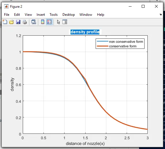
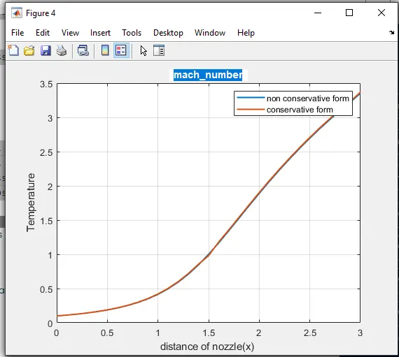
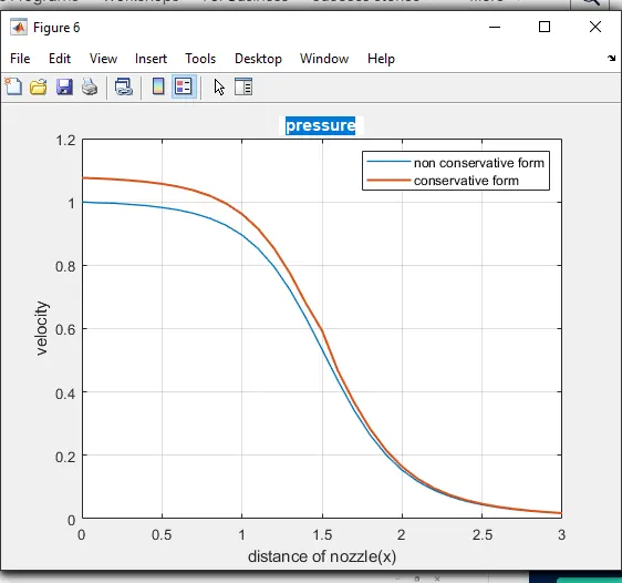
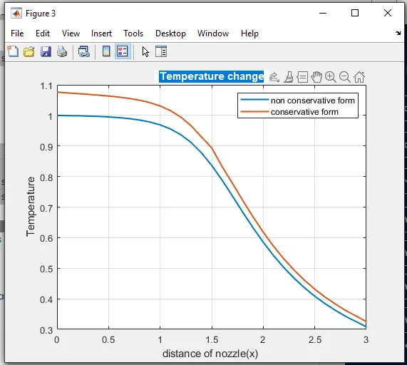
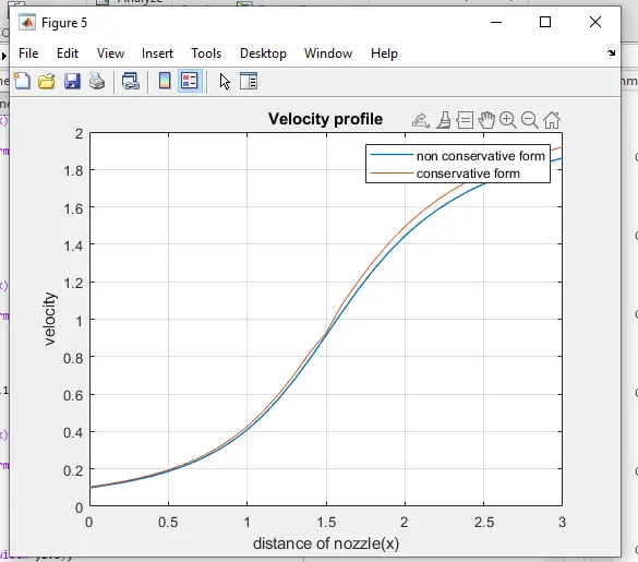
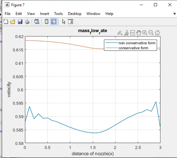
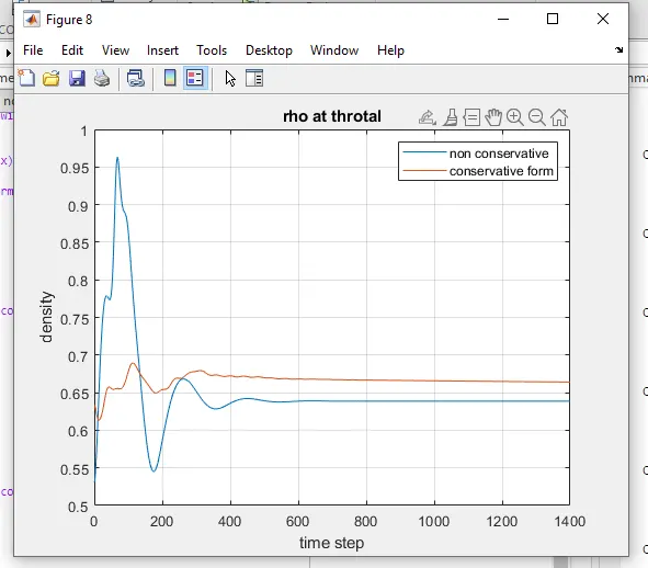
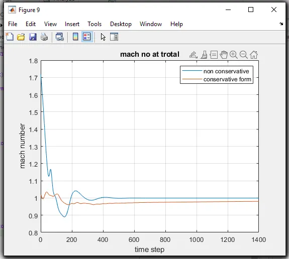
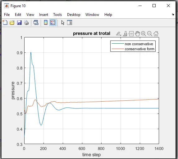
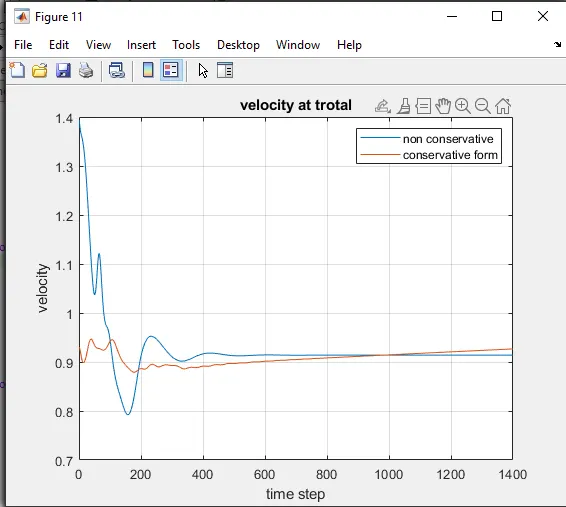
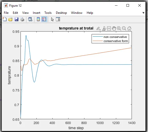
• The CFL  value does not have any effect on conservative form primate variables ratio.

• The time taken for simulation in case of conservative form is lesser as comapred to non conservative form as shown in the simulation table data.
• In grid dependence test we observe that the accuracy in case of non consevative form is more as comapared to conservative form as it is very close to exact analytical solution.
• The conservative form provides more accuracy incase of mass flow rate whereas non conservative provide more accuracy in case of primitive variables .However in general we can say that non conservative form has higher accuracy than conservative form.
• No For the first table of cfl effects signifies about the effect on non conservative form.It is observed that as CFL value increases the density,pressure and Temperature ratio increases.But however mach number decreases.For  the cfl value 1.2 the sloution gets blown off . No wonder it is the threshold CFL value . 
• In the second table it represents data for conservative form the increase or decrease in cfl value doesnt effect the solution itself.