Week 7 - Simulation of a 1D Supersonic nozzle flow simulation using Macormack Method

Aim: Simulating quasi 1-D supersonic flow through a converging diverging nozzle using MacCormack method

Objective:

• Deducing the conservative and non-conservative forms of governing equations and implementing MacCormack method to solve the equations and comparing the results.
• Computing the steady state distribution of fluid variables in the nozzle and the time variation of the variables.
• Studying the variation of mass flow rate inside the nozzle at different time steps under influence of time marching.

Theory:

A nozzle is a type of device designed to control the direction or characteristics of fluid flow at the exit of a pipe (or such system). A nozzle is often a pipe or tube of varying cross-sectional area, thus can be used to direct or modify flow of a fluid.

A convergent-divergent nozzle (also known as CD nozzle or de Laval nozzle) is a device used to accelerate a hot, pressurized gas passing through it to a higher supersonic speed in the axial direction by converting heat energy of the flow to kinetic energy. Hence, such nozzles are widely used in steam turbines, supersnic jet engines and rocket engine nozzles. Its operation relies on the different properties of gases flowing at subsonic, sonic and supersonic speeds.

In the field of CFD, MacCormack method is a prominent discretization scheme for obtaining numerical solutions of hyperbolic partial differential equations. (based on second-order finite difference method). It is the variation of two-step Lax-Wendroff scheme but much simple in application.

In this project, the problem is taken from JD Anderson's book on CFD.

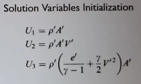
Solution vector

U1=ρ⋅a">ρ⋅a�⋅�;

U2=2*U2-U2;

U3=U1⋅((Tγ-1)+((γ2)⋅v2))">U1⋅((Tγ−1)+((γ2)⋅v2))�1⋅((��-1)+((�2)⋅�2));

Update the old solution vector and give equation for dt

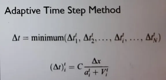
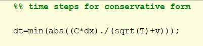
Consider u for solution vector, f for flux vector and J for source vector

Initialise flux vector for the predictor terms

Flux term

 F1=U2;

 F2=(U2.^2./U1)+((gamma-1)/gamma)*(U3-(gamma*U2.^2)./(2*U1));

 F3=(gamma*U2.*U3./U1)-(gamma*(gamma-1)/2)*(U2.^3./U1.^2);

Source term

J1=0

J2=(1γ)⋅ρ⋅T⋅dAdx">J2=(1γ)⋅ρ⋅T⋅dAdx�2=(1�)⋅�⋅�⋅����;

J3=0

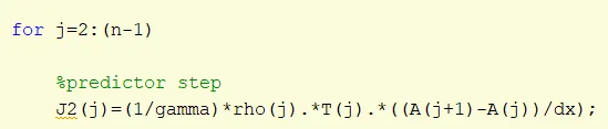
 Update the predictor solution(differential equation) using forward difference scheme

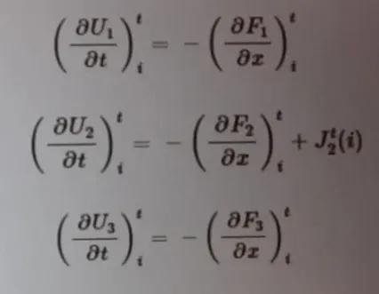
 Update the solution vector,flux vector and primitive variables using new values of predictor so as to use it in corrector step

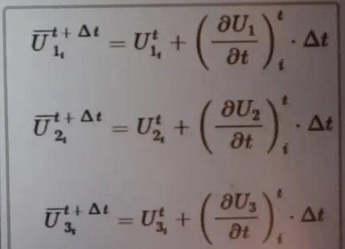
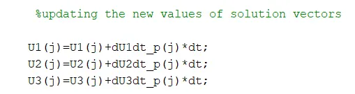
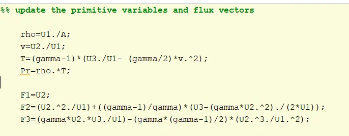
Now, go to corrector step

Use Backward difference scheme for all variables that is used in predictor method

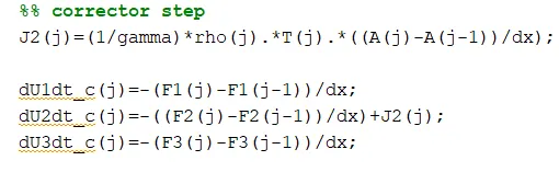
Then use the average of predictor and corrector step to update the derivatives

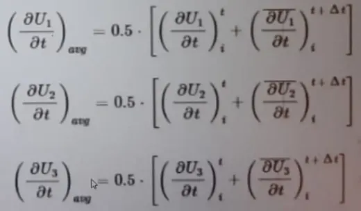
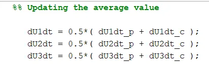
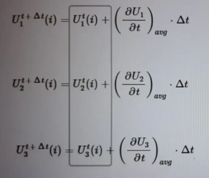
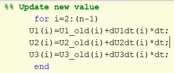
Then update the new value of solution vector at the end of each time step

Then apply boundary condition for conservative form

inlet boundary condition      

U1(1)=rho(1).*a(1);

U2(1)=2*U2(2)-U2(3);

U3(1)=U1(1)*((temp(1)/(gamma-1))+((gamma/2)*V(1).^2));

 Outlet boundary condition

  U1(n)=2*U1(n-1)-U1(n-2);

  U2(n)=2*U2(n-1)-U2(n-2);

  U3(n)=2*U3(n-1)-U3(n-2);

 After that update the primitive variable and define pressure,Mach number and mass flow rate using the updated primitive variable

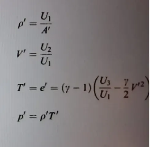
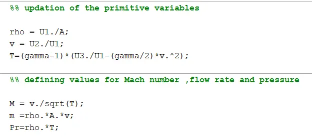
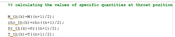
Then calculate the specific quantities at throat position.

At throat, area ratio A=1. It is at centre only.

At throat, the index is (n+1)/2;

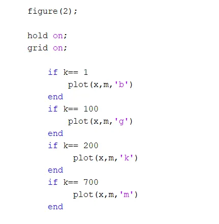
Then plot graph for mass flow rate at different time step along the length of the nozzle

Equations for Non Conservation form and coding hints

In conservation approach we consider or discretise solution in three parts are solution vector, flex vector and source vector for simplification point of view

Continuity equation

∂ρ∂t=-ρ∂v∂x-ρv∂lnA∂x-v∂ρ∂x">∂ρ∂t=−ρ∂v∂x−ρv∂lnA∂x−v∂ρ∂x∂�∂�=-�∂�∂�-��∂ln�∂�-�∂�∂�

Momentum equation

∂v∂t=-v∂v∂x-1γ(∂T∂x+Tρ∂ρ∂x)">∂v∂t=−v∂v∂x−1γ(∂T∂x+Tρ∂ρ∂x)∂�∂�=-�∂�∂�-1�(∂�∂�+��∂�∂�)

Energy equation

∂T∂t=-v∂T∂x-(γ-1)T(∂v∂x+v∂lnA∂x)">∂T∂t=−v∂T∂x−(γ−1)T(∂v∂x+v∂lnA∂x)∂�∂�=-�∂�∂�-(�-1)�(∂�∂�+�∂ln�∂�)

Define initial profile for A such that area vary as per the function of length of the nozzle 

v,T,rho are primitive variable vary as per the function of length of the nozzle 

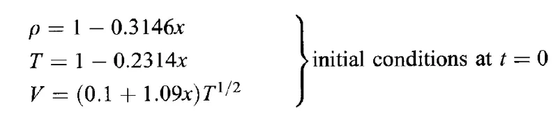
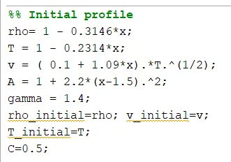
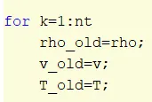
Update the old values of rho,v and T at start of every time step

Use time step formula

a=T">a=√T�=�;

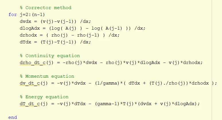
Use forward difference for predictor method and update the continuity,momentum and energy equation

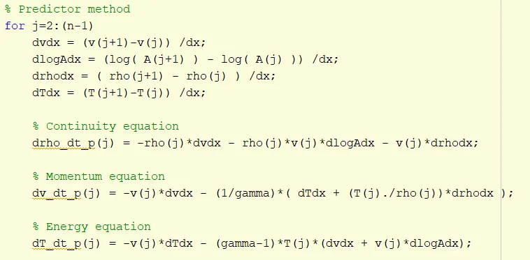
After that update the solution variable using the predictor step

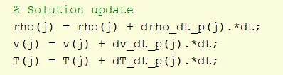
Now, go to corrector method and update theprimitive variables calculated in predictor step using backward difference scheme

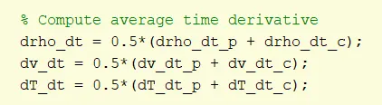
Update the solution using the average of predictor and corrector method.

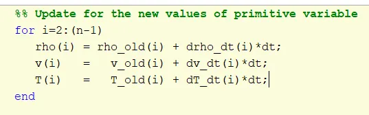
Update the new values of primitive variables

Define pressure,mach number and mass flow rate as a function of the updated primitive variables

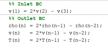
Define Inlet and Outlet boundary conditions

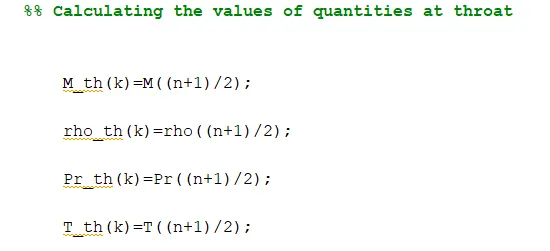
Calculate the values of Mach number, Density, Pressure, Temperature at throat

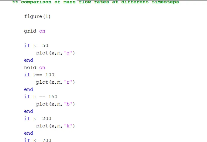
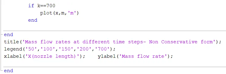
Then plot graph for mass flow rate at different time step along the length of the nozzle

 MATLAB CODE

close all; clear all;clc;

%% inputs
n=31;
x=linspace(0,3,n);
dx=x(2)-x(1);
 A = 1 + 2.2*(x-1.5).^2;
%% Output
[M,m,k,rho,T,Pr,M_th,rho_th,T_th,Pr_th,residual]=macro_non_cons(x,dx,n);
[M_c,m_c,k_c,rho_c,T_c,Pr_c,M_th_c,rho_th_c,T_th_c,Pr_th_c,residual_c] = macro_cons(x,dx,n);       

%% plot 3
    figure(3)
    
    subplot(4,1,1)
    hold on
    plot(x,M,'-');
    plot(x,M_c,'-*');
    legend('Non Conservative form','Conservative form');
    xlabel('X');    ylabel('Mach Number');
    title(sprintf('Mach Number @ Time step=%d',k));
    
    subplot(4,1,2)
    hold on
    plot(x,rho,'-');
    plot(x,rho_c,'-*');
    legend('Non Conservative form','Conservative form');
    xlabel('X');    ylabel('Density');
    title(sprintf('Density @ Time step=%d',k));

    subplot(4,1,3)
    hold on
    plot(x,T,'-');
    plot(x,T_c,'-*');
    legend('Non Conservative form','Conservative form');
    xlabel('X');    ylabel('Temperature');
    title(sprintf('Temperature @ Time step=%d',k));
    
    subplot(4,1,4)
    hold on
    plot(x,Pr,'-');
    plot(x,Pr_c,'-*');
    legend('Non Conservative form','Conservative form');
    xlabel('X');    ylabel('Pressure');
    title(sprintf('Pressure @ Time step=%d',k));
%% plot 4    
    figure(4)
    
    subplot(4,1,1)
    hold on
    plot(M_th);
    plot(M_th_c);
    legend('Non Conservative form','Conservative form');
    xlabel('Time Step');    ylabel('Mach Number');
    title(sprintf('Mach Number at centre for all Time step'));
    
    subplot(4,1,2)
    hold on
    plot(rho_th);
    plot(rho_th_c);
    legend('Non Conservative form','Conservative form');
    xlabel('Time Step');    ylabel('Density');
    title(sprintf('Density at centre for all Time step'));

    subplot(4,1,3)
    hold on
    plot(T_th);
    plot(T_th_c);
    legend('Non Conservative form','Conservative form');
    xlabel('Time Step');    ylabel('Temperature');
    title(sprintf('Temperature at centre for all Time step'));
    
    subplot(4,1,4)
    hold on
    plot(Pr_th);
    plot(Pr_th_c);
    legend('Non Conservative form','Conservative form');
    xlabel('Time Step');    ylabel('Pressure');
    title(sprintf('Pressure at centre for all Time step'));
    
%% plot 5
figure(5)
subplot(2,1,1)
    hold on
    plot(residual);
    title('Residual:Non Conservative form');
    xlabel('Time Step');    ylabel('Residual');
    legend('drho/dt','dv/dt','dT/dt');
    
subplot(2,1,2)
    hold on
    plot(residual_c);
    title('Residual:Conservative form');
    xlabel('Time Step');    ylabel('Residual');
    legend('dU1/dt','dU2/dt','dU3/dt');    
%% plot 6
figure(6)
plot(x,m);
hold on
plot(x,m_c);
xlabel('X(nozzle length)');
ylabel('Mass flow rate');
title('Mass flow rate at the end of time step in Non Conservative and Conservative form');
legend('Non Conservative form','Conservative form');

 Non conservative form function

function[M,m,k,rho,T,Pr,M_th,rho_th,T_th,Pr_th,residual] = macro_non_cons(x,dx,n)



%% Initial profile
rho= 1 - 0.3146*x;
T = 1 - 0.2314*x;
v = ( 0.1 + 1.09*x).*T.^(1/2);
A = 1 + 2.2*(x-1.5).^2;
gamma = 1.4;
rho_initial=rho; v_initial=v;
T_initial=T;
C=0.5;

%% Time step
nt=1400;
dt=0.01;

for k=1:nt
    rho_old=rho;
    v_old=v;
    T_old=T;
    
    dt=min(abs(C.*dx./(sqrt(T)+v)));
    % Predictor method
    for j=2:(n-1)
        dvdx = (v(j+1)-v(j)) /dx;
        dlogAdx = (log( A(j+1) ) - log( A(j) )) /dx;
        drhodx = ( rho(j+1) - rho(j) ) /dx;
        dTdx = (T(j+1)-T(j)) /dx;
        
        % Continuity equation
        drho_dt_p(j) = -rho(j)*dvdx - rho(j)*v(j)*dlogAdx - v(j)*drhodx;
        
        % Momentum equation
        dv_dt_p(j) = -v(j)*dvdx - (1/gamma)*( dTdx + (T(j)./rho(j))*drhodx );
        
        % Energy equation
        dT_dt_p(j) = -v(j)*dTdx - (gamma-1)*T(j)*(dvdx + v(j)*dlogAdx);
        
            % Solution update
            rho(j) = rho(j) + drho_dt_p(j).*dt;
            v(j) = v(j) + dv_dt_p(j).*dt;
            T(j) = T(j) + dT_dt_p(j).*dt;
    end

        % Corrector method
    for j=2:(n-1)
        dvdx = (v(j)-v(j-1)) /dx;
        dlogAdx = (log( A(j) ) - log( A(j-1) )) /dx;
        drhodx = ( rho(j) - rho(j-1) ) /dx;
        dTdx = (T(j)-T(j-1)) /dx;
        
        % Continuity equation
        drho_dt_c(j) = -rho(j)*dvdx - rho(j)*v(j)*dlogAdx - v(j)*drhodx;
            
        % Momentum equation
        dv_dt_c(j) = -v(j)*dvdx - (1/gamma)*( dTdx + (T(j)./rho(j))*drhodx );
        
        % Energy equation
        dT_dt_c(j) = -v(j)*dTdx - (gamma-1)*T(j)*(dvdx + v(j)*dlogAdx);
        
    end
    
    % Compute average time derivative
    drho_dt = 0.5*(drho_dt_p + drho_dt_c);
    dv_dt = 0.5*(dv_dt_p + dv_dt_c);
    dT_dt = 0.5*(dT_dt_p + dT_dt_c);
    
    residual(k,1) = max(abs(drho_dt));
    residual(k,2) = max(abs(dv_dt));
    residual(k,3) = max(abs(dT_dt));
    
    %% Update for the new values of primitive variable
    for i=2:(n-1)
       rho(i) = rho_old(i) + drho_dt(i)*dt;
       v(i)   =   v_old(i) + dv_dt(i)*dt;
       T(i)   =   T_old(i) + dT_dt(i)*dt;
    end
    
   %% Define pressure,mach number and mass flow rate 
    Pr = rho.*T;
    M = v./sqrt(T);
    m = rho.*A.*v;
    %% Inlet BC
    v(1) = 2*v(2) - v(3);
    %% Outlet BC
    rho(n) = 2*rho(n-1) - rho(n-2);
    v(n)   = 2*v(n-1) - v(n-2);
    T(n)   = 2*T(n-1) - T(n-2);
    
    %% Calculating the values of quantities at throat

    
        M_th(k)=M((n+1)/2);

        rho_th(k)=rho((n+1)/2);

        Pr_th(k)=Pr((n+1)/2);

        T_th(k)=T((n+1)/2);
 
    %% comparison of mass flow rates at different timesteps

        figure(1)

        grid on
              
        if k==50
            plot(x,m,'g')
        end
        hold on
        if k== 100
            plot(x,m,'r')
        end
        if k == 150
            plot(x,m,'b')
        end
        if k==200
            plot(x,m,'k')
        end
        if k==700
            plot(x,m,'m')
        end
    
end
title('Mass flow rates at different time steps- Non Conservative form');
legend('50','100','150','200','700');
xlabel('X(nozzle length)');    ylabel('Mass flow rate');

end

Conservative form function

function[M,m,k,rho,T,Pr,M_th,rho_th,T_th,Pr_th,residual] = macro_cons(x,dx,n)


%% Time step
nt=1400;
dt=0.01;

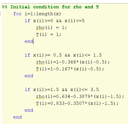
%% Initial condition for rho and T
    for i=1:length(x)
        if x(i)>=0 && x(i)<=5
            rho(i) = 1;
            T(i) = 1;
        end
    
        if x(i)>= 0.5 && x(i)<= 1.5
            rho(i)=1-0.366*(x(i)-0.5);
            T(i)=1-0.167*(x(i)-0.5);
        end
        
        if x(i)>=1.5 && x(i)<= 3.5
            rho(i)=0.634-0.3879*(x(i)-1.5);
            T(i)=0.833-0.3507*(x(i)-1.5);
        end
    end
    
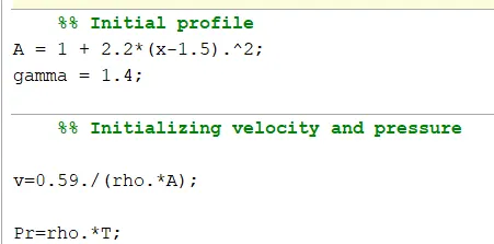
    %% Initial profile
A = 1 + 2.2*(x-1.5).^2;
gamma = 1.4;
    
    %% Initializing velocity and pressure

v=0.59./(rho.*A);

Pr=rho.*T;

rho_initial=rho; v_initial=v;
T_initial=T;
C=0.5;
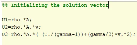
%% Initializing the solution vector

U1=rho.*A;
U2=rho.*A.*v;
U3=rho.*A.*( (T./(gamma-1))+(gamma/2)*v.^2);

for k=1:nt
    %% updating old solution vectors

    U1_old=U1;
    U2_old=U2;
    U3_old=U3;
    %% time steps for conservative form

    dt=min(abs((C*dx)./(sqrt(T)+v)));

    %% predictor
    F1 = U2;
    F2 = (U2.^2)./U1 + ((gamma-1)/gamma)*( U3 - (gamma/2)*(U2.^2)./U1 );
    F3 = gamma*U2.*U3./U1 - (gamma*(gamma-1)/2)*(U2.^3)/(U1.^2);
    
    
    for j=2:(n-1)
        
        %predictor step
        J2(j)=(1/gamma)*rho(j).*T(j).*((A(j+1)-A(j))/dx);
        
        
        dU1dt_p(j)=-(F1(j+1)-F1(j))/dx;
        dU2dt_p(j)=-((F2(j+1)-F2(j))/dx)+J2(j);
        dU3dt_p(j)=-(F3(j+1)-F3(j))/dx;
        
         %updating the new values of solution vectors

        U1(j)=U1(j)+dU1dt_p(j)*dt;
        U2(j)=U2(j)+dU2dt_p(j)*dt;
        U3(j)=U3(j)+dU3dt_p(j)*dt;
        
    end


%% update the primitive variables and flux vectors

    rho=U1./A;
    v=U2./U1;
    T=(gamma-1)*(U3./U1- (gamma/2)*v.^2);
    Pr=rho.*T;

    F1=U2;
    F2=(U2.^2./U1)+((gamma-1)/gamma)*(U3-(gamma*U2.^2)./(2*U1));
    F3=(gamma*U2.*U3./U1)-(gamma*(gamma-1)/2)*(U2.^3./U1.^2);

    %%
    for j=2:(n-1)
        
        %% corrector step
        J2(j)=(1/gamma)*rho(j).*T(j).*((A(j)-A(j-1))/dx);
        
        dU1dt_c(j)=-(F1(j)-F1(j-1))/dx;
        dU2dt_c(j)=-((F2(j)-F2(j-1))/dx)+J2(j);
        dU3dt_c(j)=-(F3(j)-F3(j-1))/dx;
        
    end
     %% Updating the average value

        dU1dt = 0.5*( dU1dt_p + dU1dt_c );
        dU2dt = 0.5*( dU2dt_p + dU2dt_c );
        dU3dt = 0.5*( dU3dt_p + dU3dt_c );
        residual(k,1) = max(abs(dU1dt));
        residual(k,2) = max(abs(dU2dt));
        residual(k,3) = max(abs(dU3dt));
  %% Update new value      
        for i=2:(n-1)
       U1(i)=U1_old(i)+dU1dt(i)*dt;
       U2(i)=U2_old(i)+dU2dt(i)*dt;
       U3(i)=U3_old(i)+dU3dt(i)*dt;
        end
    
    %% applying BC

        %% inlet BC

        U1(1)=rho(1).*A(1);
        U2(1)=2*U2(2)-U2(3);
        U3(1)=U1(1).*((T(1)/(gamma-1))+((gamma/2)*v(1).^2));
       
        %% Outlet BC

        U1(n)=2*U1(n-1)-U1(n-2);
        U2(n)=2*U2(n-1)-U2(n-2);
        U3(n)=2*U3(n-1)-U3(n-2);
        
        %% updation of the primitive variables

        rho = U1./A;
        v = U2./U1;
        T=(gamma-1)*(U3./U1-(gamma/2)*v.^2);

        %% defining values for Mach number ,flow rate and pressure

        M = v./sqrt(T);
        m =rho.*A.*v;
        Pr=rho.*T;
        
        %% calculating the values of specific quantities at throat position

        M_th(k)=M((n+1)/2);
        rho_th(k)=rho((n+1)/2);
        Pr_th(k)=Pr((n+1)/2);
        T_th(k)=T((n+1)/2);
        %% comparison mass flow rates at different timesteps

        figure(2);

        hold on;
        grid on;

            if k== 1
                plot(x,m,'b')
            end
            if k== 100
                plot(x,m,'g')
            end
            if k== 200
                 plot(x,m,'k')
            end
            if k== 700
                 plot(x,m,'m')
            end


end
title('Mass flow rates at different time steps- Conservative form');
legend('1','100','200','700');
xlabel('X(nozzle length)');    ylabel('mass flow rate');

end

OUTPUT

1) At n=31

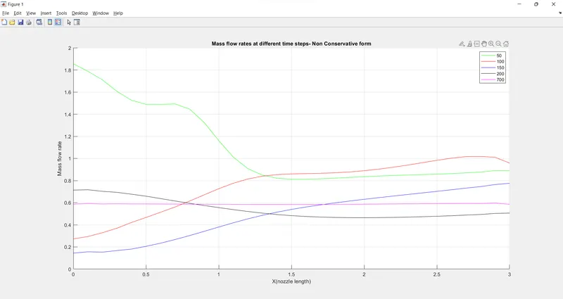
a)Mass flow rates at different time steps- Non Conservative form

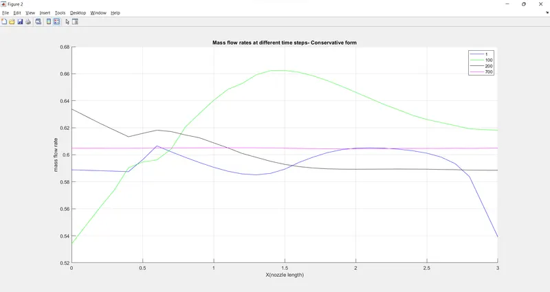
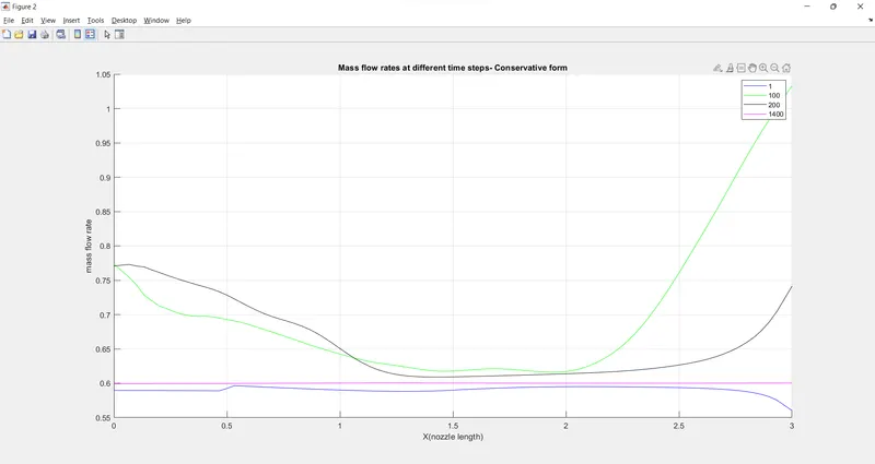
b)Mass flow rates at different time steps- Conservative form

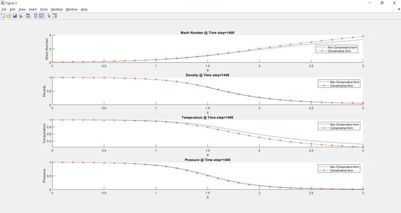
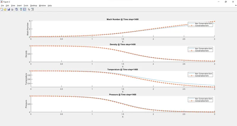
c) Mach number, Density, Pressure, Temperature variation along X axis after the end of time step

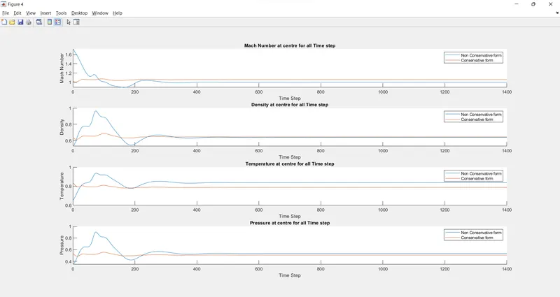
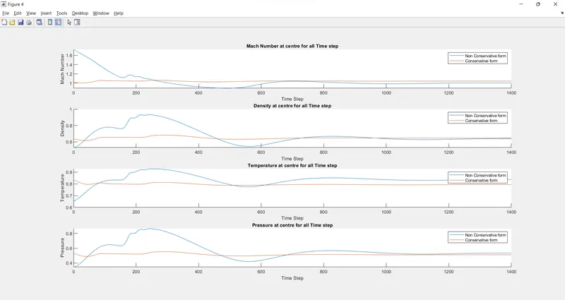
d) Mach number, Density, Pressure, Temperature at throat after each timestep

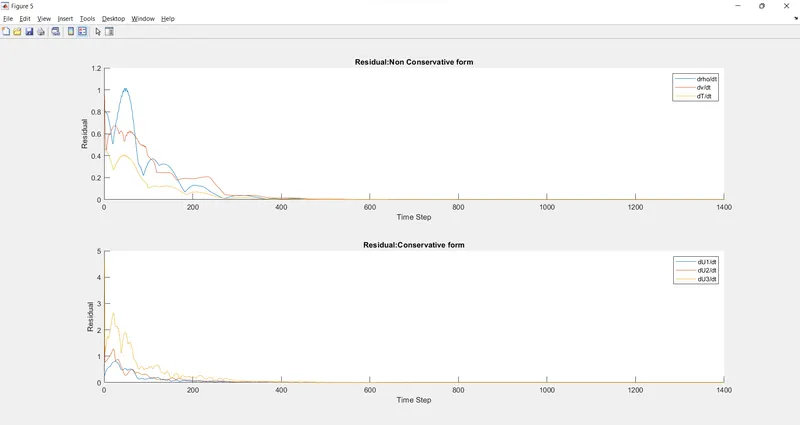
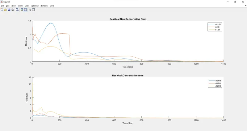
e) Residuals at exit at every time step

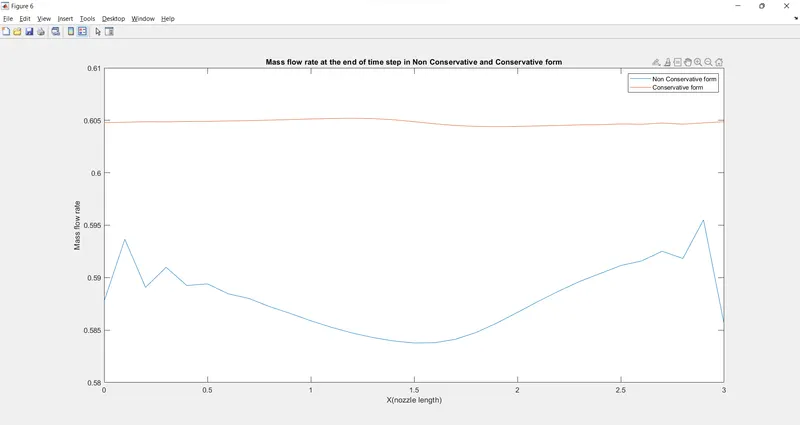
f) Mass flow rates at different time steps- Non Conservative form

CONCLUSION

From figure a and figure b, it is noticed that the mass flow rate attains steady state nearly at 700 time step. The variation gets reduced from 0 to 700 time step.

From figure c, it is observed that the values of Mach Number, Pressure, Density and Temperature are almost same from both conservative and non conservative form of governing equation.

From figure d, it is observed that the values of Mach Number, Pressure, Density and Temperature attained steady state quicker in conservative form than that of in non conservative form. The variation is small

 Figure e is just a residual plot at the nozzle exit at every time step

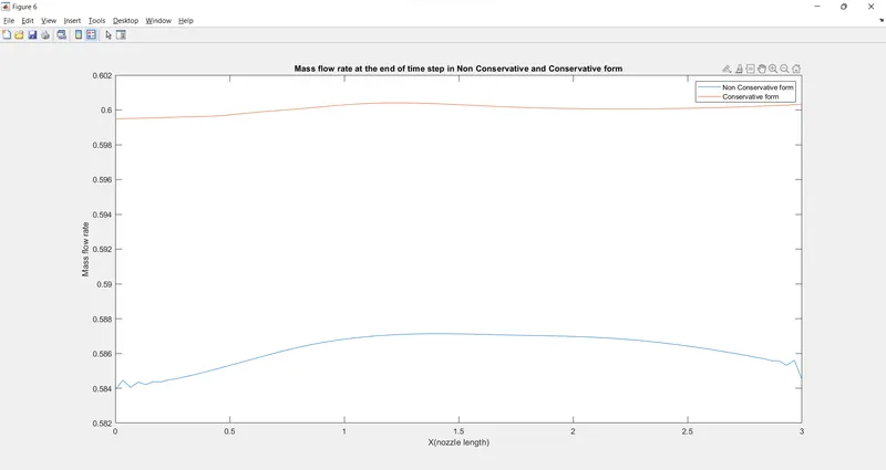
Figure f shows that the mass flow rate at the end of simulation is nearly constant in conservative form and it is varying in between 0.585 to 0.595 in non - conservative form

2) At n=91

a)Mass flow rates at different time steps- Non Conservative form

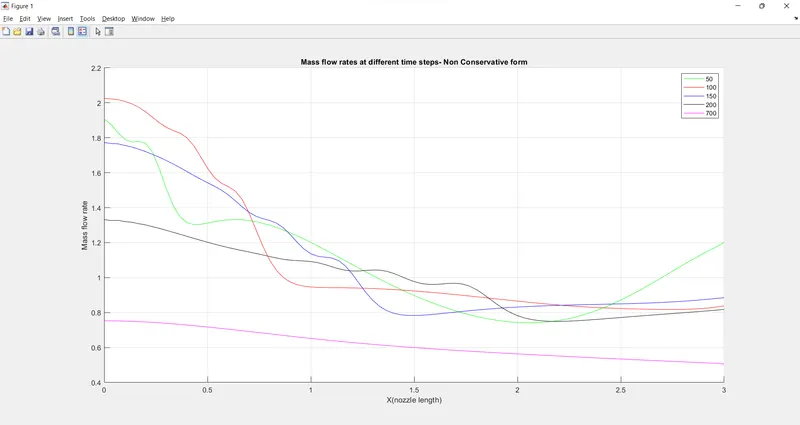
Use 1400 instead of 700

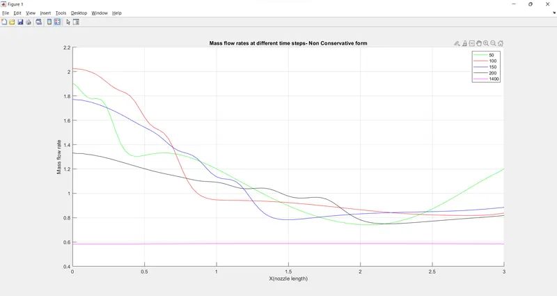
b)Mass flow rates at different time steps- Conservative form

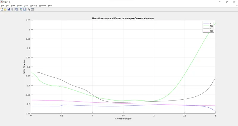
Use 1400 instead of 700

c) Mach number, Density, Pressure, Temperature variation along X axis after the end of time step

d) Mach number, Density, Pressure, Temperature at throat after each timestep

e) Residuals at exit at every time step

f) Mass flow rates at different time steps- Non Conservative form

CONCLUSION

From figure a and figure b, it is found that as the mesh size reduced, it takes more time to attain steady state. At 700 time step, the solution has not reached steady state, when compared to case at n=31.

From figure d, it is found that, it takes more time for non conservative form to attain steady state at throttle area, but for conservative form, it attains steady state faster irrespective of mesh size

From figure f, it is found that for non conservative form, there is not much variation in mass flow rate at outlet when compared to case at n=31. For conservative form, the value is not changing with the length of the nozzle

% witting program for simulation of 1D NOZZEL SUPERSONIC FLO USING MACORMAC
%METHOD 
clear all
close all 
clc

%defing the inputs 
%number of grids points 
n=31
x=linspace(0,3,n);
dx=x(2)-x(1);


gamma=1.4;

%number of time steps
nt=1400;
CFL=0.5;

%defing the function for non conservation form of simulation 
tic;
[mass_flow_rate_nc,presure_nc,mach_num_nc,rho_nc,v_nc,T_nc,rho_trottle_nc,v_trottle_nc.T_trottle_nc,mass_flow_rate_trottle_nc,presure_trottle_nc,mach_num_trottle_nc]=non_conservative_form_original(x,dx,n,gamma,nt,CFL)
time_elapsed=toc;
fprintf('time elapesed for non coservation form.%f',time_elapsed)
hold on 
%ploting the graphs
figure(3)
%for density
subplot(4,1,1)
plot(linspace(1,nt,1400),rho_trottle_nc,"color","m");
ylabel("density")
legend({'density at trottle'})
title('timestep variation at trottle area-non conservation form')

%for tempreture
subplot(4,1,2)
plot(linspace(1,nt,1400),T_trottle_nc,"color","b");
ylabel("tempreture")
legend({'tempreture at trottle'})
title('timestep variation at trottle area-non conservation form')

%for presure
subplot(4,1,3)
plot(linspace(1,nt,1400),presure_trottle_nc,"Color","r");
ylabel("presure")
legend({'presure at trottle'})
title('timestep variation at trottle area-non conservation form')

%for mach number
subplot(4,1,4)
plot(linspace(1,nt,1400),mach_num_trottle_nc,"Color","m");
xlable('time step')
ylable("mach number")
legend({'mach num at trottle'})
title('timestep variation at trottele area-non conservation form')

%for tempreture
subplot(4,1,2)
plot(x,T_nc,"Color",