Week 4.1 - Genetic Algorithm

AIM:-GENETIC ALGORRTHM

OBJECTIVE:- To optimese the stalagmite function and find the global maxima of the function by using MATLAB

Genetic Algorithm:-

Genetic algorithm (GA) is a branch of field of study called evolutionary comutation it is based on evolution theory by darwin GA is used to optimize a given function to find its maximum or mininmum value.the basic components of a GA are

1. Fitness function it is the function that GA is trying to optimize

2. A population of chromosome it is the numerical valus that represent all the solution to the function the selection operator chooses some of the chromosomes (with replacement)for reproduction based on probability distributon.fitter the chromosome more likely it is to be selected

3. cross over this operator swaps in random a subsequence of two of the chosen chromosomes tocreate two offspring usually each chromosome is converted into binary code and then cross over is done from one parent chromosome into another.

x ga(fun,nvars,a,b,aeq,beq,lb,ub,nonlcon,intcon,option)

where

fun = objective function

nvars = number of variables

A and B = subject to linear lnequalities of the form A*x <=B

Aeq and Beq = subject to linear equalities of the form A*x=B

LB = lower bound

UB = upper bound

nonlcon = Nonlinear constraints

options = Optimization options

FUNCTION CODE:-

function [P]= gene_alg(input_vector)
x = input_vector(1);
y = input_vector(2);
f1x=(sin((5.1*pi*x)+0.5))^6;
fly=(sin((5.1*pi*y)+0.5))^6;
t1 = ((x-0.0667).^2/(0.64));
t2  = ((y-0.0667).^2/(0.64));
f2x = exp(-4*log(2)*t1);
f2y = exp(-4*log(2)*t2);
P = -(f1x.*f2x.*fly.*f2y);
end

MAIN CODE:-

clear all 
close all
clc


% search space for the function.
x = linspace(0,1,350);
y = linspace(0,1,350);


% use of meshgrid command to get 2D arrays.
[xx yy] = meshgrid(x,y);

% Number of iteration performed by the function.
num_case = 150

% surface plot for genetic algorithm function
for i = 1:length(xx)
end

for j = 1:length(yy);
    input_vector(1) = xx(i,j);
    input_vector(2) = yy(i,j);
    p(i,j) = gene_alg(input_vector);
end

% Generate the surface for the plot.
surfc(xx,yy,-p);

% Remove the line produce by meshgrid
shading interp

% Initiate timer for calculating survey time.
tic
for i = 1:num_case
    % calculate the optimized value of the function.
    [inputs,popt(i)] = ga(@gene_alg,2);
    % Optimised value at ech iterations.
    xopt(i) = inputs(1);
    yopt(i) = inputs(2);
end

% Display time taken to complete the survey.
survey1_time = toc

% plot the graph with the obtained optimized data.
figure(1)
subplot(2,1,1)
surfc(xx,yy,-p);
hold on
shading interp
plot3(xopt,yopt,-popt,'marker','o','markersize',5,'MarkerFaceColor','g');
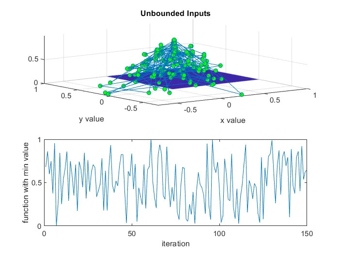
title('Unbounded Inputs');
xlabel('x value');
ylabel('y value');
grid on
 subplot(2,1,2)
plot(-popt);
xlabel('iteration');
ylabel('function with min value');

% Initiate timer for calulating survey time.
tic
for j = 1:num_case
    % Calculate the optimized value of the function.
    [inputs,popt(j)] = ga(@gene_alg,2,[],[],[],[],[0;0],[1;1]);
    % Optimised value at ech iteration.
    xopt(j) = inputs(1);
    yopt(j) = inputs(2);
end

% Display time taken to complete the survey.
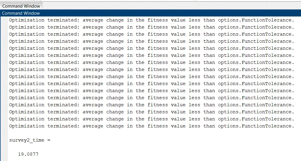
survey2_time = toc

% plot the graph with obtained optimized data.
figure(2)
subplot(2,1,1)
surfc(xx,yy,-p);
hold on
shading interp
plot3(xopt,yopt,-popt,'Marker','0','Markersize',5,'MarkerFacecolor','g');
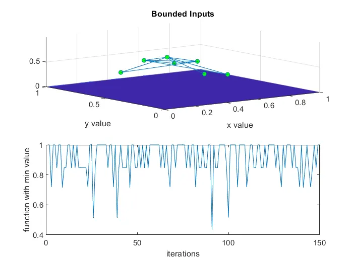
title('Bounded Inputs');
xlabel('x value');
ylabel('y value');
grid on
subplot(2,1,2)
plot(-popt);
xlabel('iterations');
ylabel('function with min value');

% Initiate timer for calulating survey time.
tic
for k = 1:num_case
    % Calculate the optimized value of the function.
    [inputs,popt(k)] = ga(@gene_alg,2,[],[],[],[],[0;0],[1;1],[],[],options);
    % Optimised value at ech iteration.
    xopt(k) = inputs(1);
    yopt(k) = inputs(2);
end

% Display time taken to complete the survey.
survey3_time = toc
% plot the graph with the obtained optimized data.
figure(3)
subplot(2,1,1)
surfc(xx,yy,-p);
hold on
shading interp
plot3(xopt,yopt,-popt,'Marker','0','Markersize',5,'Markerfacecolor','g');
title('statistical study with increase in population');
xlabel('x value');
ylabel('y value');
grid on
subplot(2,1,2)
plot(-popt);
xlabel('iteration');
ylabel('function with min value');

OUTPUTS IN WORKSPACE :-

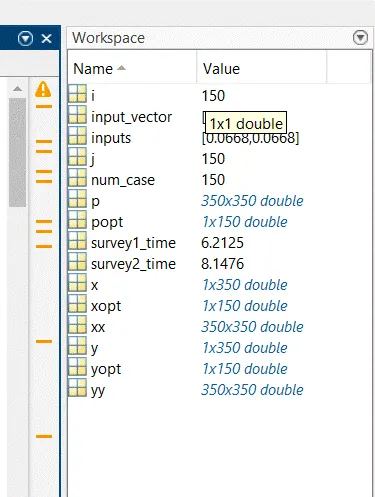
unbounded inputs:-