Week 7 - Simulation of a 1D Super-sonic nozzle flow simulation using Macormack Method
CHALLENGE - 7 : Simulation of a 1D Super-Sonic Nozzle Flow Simulation using Macormack Method
AIM:
To write a Matlab program to simulate the isentropic flow through a quasi 1D subsonic-supersonic nozzle by both the conservation and non-conservation forms of the governing equations and to solve them using the MacCormack's technique.
OBJECTIVE:
- To write a Matlab program to simulate the isentropic flow through a quasi 1D subsonic-supersonic nozzle.
- To solve the problem by MacCormack's technique considering both the conservation and non-conservation forms of the governing equations.
- To plot steady state distribution and time wise variation of primitive variables inside the nozzle.
- To compare the mass flow rate at steady state for both conservation form and non-conservation form.
- To plot the variation of Mass flow rate distribution inside the nozzle at different time steps during the time-marching process.
- To perform a grid independence test on the solution.
THEORY & EQUATIONS USED:
- Non-Conservation form
Continuity eqaution:
`(delrho)/(delt)=-rho(delV)/(delx)-rhoV(dellnA)/(delx)-V(delrho)/(delx)`
Momentum Equation:
`(delV)/(delt)=-V(delV)/(delx)-1/gamma((delT)/(delx)+T/rho(delrho)/(delx))`
Energy Equation:
`(delT)/(delt)=-V(delT)/(delx)-(gamma-1)T((delV)/(delx)+V(del(lnA))/(delx))`
Initial Conditions (t = 0)
`rho=1-0.3146x`
`T = 1-0.2314x`
`V = (0.1+1.09x)T^(1/2)`
Nozzle shape `A = 1+2.2(x-1.5)^2`
Boundary conditions
Inlet:- Two variables are fixed and one variable float that is density and temperature is fixed and velocity is float.
therefore:
`V_1 = 2V_2-V_3`
Outlet: All the three variables are float.
`V_N = 2V_(N-1)-V_(N-2)`
`rho_N = 2rho_(N-1)-rho_(N-2)`
`T_N = 2T_(N-1)-T_(N-2)`
- Conservation form
Continuity eqaution:
`(del(rhoA))/(delt)+(del(rhoAV))/(delx)=0`
Momentum Equation:
`(del(rhoAV))/(delt)+(del(rhoAV^2+(1/gamma)pA))/(delx)=1/gammap(delA)/(delx)`
Energy Equation:
`(del(rho(T/(gamma-1)+gamma/2V^2)A))/(delt)+(del(rho(T/(gamma-1)+gamma/2V^2)AV+pAV))/(delx)=0`
Lets define the elements of the solutions vector U, the flux vector F and the source term J as follows
`U_1 = rhoA`
`U_2=rhoAV`
`U_3 = rho(T/(gamma-1)+gamma/2V^2)A`
`F_1 = rhoAV`
`F_2 = rhoAV^2+1/gammapA`
`F_3 = rho(T/(gamma-1)+gamma/2V^2)VA+pAV`
`J_2 = 1/gammap(delA)/(delx)`
By using these elements the continuity, the momentum and the energy equation is rewritten as
`(delU_1)/(delt)=-(delF_1)/(delx)`
`(delU_2)/(delt)=-(delF_2)/(delx)+J_2`
`(delU_3)/(delt)=-(delF_3)/(delx)`
Initial Conditions (t = 0)
`[[rho=1],[T=1]]} "for " 0<=x<=0.5`
`[[rho=1-0.366(x-0.5)],[T=1-0.167(x-0.5)]]} "for " 0.5<=x<=1.5`
`[[rho=0.634-0.3879(x-1.5)],[T=0.833-0.3507(x-1.5)]]} "for " 1.5<=x<=3.5`
`V = 0.59/(rhoA)`
Nozzle shape `A = 1+2.2(x-1.5)^2`
Boundary conditions
Inlet:- Two variables are fixed and one variable float that is density and temperature is fixed and velocity is float.
therefore:
`U_2(i=1) = 2U_2(i=2)-U_2(i=3)`
U3 is also updated by using the value of updated V.
Outlet: All the three variables are float.
`(U_1)_N = 2(U_1)_(N-1)-(U_1)_(N-2)`
`(U_2)_N = 2(U_2)_(N-1)-(U_2)_(N-2)`
`(U_3)_N = 2(U_3)_(N-1)-(U_3)_(N-2)`
PROCEDURE:
Procedure for matlab program is mentioned below.
- Program is started by using the general commands clear all, close all and clc to clear and close all the pre-occupied operations of Matlab.
- Provide the input data.
- call the functions to perform the simulation using non conservation form and conservation form. By using the above mentioned eqautions and with the help of MacCormack's technique the problem is solved.
- Plot the comparison graphs mentioned as mentioned in the objective session.
- Save and Run the file.
The main program is attached below.
% Simulation of a 1D Super-sonic nozzle flow simulation using Macormack Method
close all
clear all
clc

n = 91;
x= linspace(0,3,n);
dx = x(2)-x(1);
nt = 1400;
gamma = 1.4;

% Function call
[mdot_nc] = non_cons(n, x, dx, nt, gamma);
[mdot_c] = cons(n, x, dx, nt, gamma);

% Plotting Mass flow rate
figure(7)
plot(x,mdot_nc(end,:), '-r')
hold on
plot(x,mdot_c(end,:), '-k')
xlabel('Nozzle Length');
ylabel('Massflow Rate')
legend('Non conservative form', 'Conservative form')
title('Comparison of steady state mass flow rate distributions of both forms')- Function script for Non-Conservation form
% Function for non-conservative form
function [mdot] = non_cons(n, x, dx, nt, gamma)

% initializing the varibales
rho = 1-(0.3146*x);
t = 1-(0.2314*x);
v = (0.1+(1.09*x)).*t.^0.5;
a = (1+2.2*(x-1.5).^2);
throat = find(a==1);

dt = min(0.5*dx./(t.^0.5+v));

% looping starts here
for k = 1:nt

    rho_old = rho;
    t_old = t;
    v_old = v;

    % Predictor
    for j = 2:n-1

        dvdx = (v(j+1)-v(j))/dx;
        drhodx = (rho(j+1)-rho(j))/dx;
        dtdx = (t(j+1)-t(j))/dx;
        dloga_dx = (log(a(j+1))-log(a(j)))/dx;

        drhodt_p(j) = -(rho(j)*dvdx)-(rho(j)*v(j)*dloga_dx)-(v(j)*drhodx);
        dvdt_p(j) = -(v(j)*dvdx)-(1/gamma)*((dtdx)+(t(j)/rho(j))*drhodx);
        dtdt_p(j) = -(v(j)*dtdx)-((gamma-1)*t(j)*(dvdx+(v(j)*dloga_dx)));

        % Solution Update
        rho(j) = rho(j)+(drhodt_p(j)*dt);
        v(j) = v(j)+(dvdt_p(j)*dt);
        t(j) = t(j)+(dtdt_p(j)*dt);
    end

    % Corrector
    for j = 2:n-1

        dvdx = (v(j)-v(j-1))/dx;
        drhodx = (rho(j)-rho(j-1))/dx;
        dtdx = (t(j)-t(j-1))/dx;
        dloga_dx = (log(a(j))-log(a(j-1)))/dx;

        drhodt_c(j) = -rho(j)*dvdx-rho(j)*v(j)*dloga_dx-v(j)*drhodx;
        dvdt_c(j) = -v(j)*dvdx-(1/gamma)*((dtdx)+(t(j)/rho(j))*drhodx);
        dtdt_c(j) = -v(j)*dtdx-(gamma-1)*t(j)*(dvdx+(v(j)*dloga_dx));

    end

    % Average
    drhodt = 0.5*(drhodt_p+drhodt_c);
    dvdt = 0.5*(dvdt_p+dvdt_c);
    dtdt = 0.5*(dtdt_p+dtdt_c);

    % Final Solution Update
    for i =2:n-1
        rho(i) = rho_old(i)+drhodt(i)*dt;
        v(i) = v_old(i)+dvdt(i)*dt;
        t(i) = t_old(i)+dtdt(i)*dt;
    end

    % Boundary condition
    % Inlet
    v(1) = 2*v(2)-v(3);

    % Outlet
    v(n) = 2*v(n-1)-v(n-2);
    rho(n) = 2*rho(n-1)-rho(n-2);
    t(n) = 2*t(n-1)-t(n-2);

    p = rho.*t;
    mach = v./(t.^0.5);
    mdot(k,:) = rho.*a.*v;

    % Varibales at throat
    mach_throat(k) = mach(throat);
    p_throat(k) = p(throat);
    t_throat(k) = t(throat);
    rho_throat(k) = rho(throat);


end

% Plotting
figure(1)
subplot(4,1,1)
plot(x, p, '-r')
title('Steady-state distribution of primitive variables inside the nozzle (Nondimensional) (Non-Conservative form)')
xlabel('Nozzle Length')
ylabel('Pressure')
subplot(4,1,2)
plot(x, rho, '-b')
xlabel('Nozzle Length')
ylabel('Density')
subplot(4,1,3)
plot(x, t, '-k')
xlabel('Nozzle Length')
ylabel('Temperature')
subplot(4,1,4)
plot(x, mach, '-g')
xlabel('Nozzle Length')
ylabel('Mach Number')

figure(2)
subplot(4,1,1)
plot(1:nt, rho_throat, '-r')
title('Time-wise variation of the primitive variables (Nondimensional) at Throat (Non-Conservative form)')
xlabel('Time Step')
ylabel('Density')
subplot(4,1,2)
plot(1:nt, t_throat, '-b')
xlabel('Time Step')
ylabel('Temperature')
subplot(4,1,3)
plot(1:nt, p_throat, '-k')
xlabel('Time Step')
ylabel('Pressure')
subplot(4,1,4)
plot(1:nt, mach_throat, '-g')
xlabel('Time Step')
ylabel('Mach Number')

figure(3)
plot(x,mdot(50,:))
hold on
plot(x,mdot(100,:))
hold on
plot(x,mdot(200,:))
hold on
plot(x,mdot(600,:))
hold on
plot(x,mdot(1400,:))
xlabel('Nozzle Length')
ylabel('Mass-flow rate')
title('Variation of Mass flow rate (Nondimensional) distribution inside the nozzle at different time steps (Non-Conservative form)')
legend('Time Step = 50','Time Step = 100','Time Step = 200','Time Step = 600','Time Step = 1400')

end
- Function script for Conservation form
% Function for conservative form
function [mdot] = cons(n, x, dx, nt, gamma)


% initializing the varibales
for i = 1:n
    if (x(i)>= 0 && x(i)<0.5)
        rho(i) = 1;
        t(i) = 1;
    elseif (x(i)>= 0.5 && x(i)<1.5)
             rho(i) = 1-0.366*(x(i)-0.5);
             t(i) = 1-(0.167*(x(i)-0.5));
    elseif (x(i)>= 1.5 && x(i)<=3.5)
             rho(i) = 0.634-(0.3879*(x(i)-1.5));
             t(i) = 0.833-(0.35*(x(i)-1.5));

    end

end
a = 1+2.2*(x-1.5).^2;
cfl = 0.5;
v = (0.59)./(rho.*a);
dt = min(cfl*dx./(t.^0.5+v));
throat = find(a==1);
    u1 = rho.*a;
    u2 = rho.*a.*v;
    u3 = rho.*a.*(t./(gamma-1))+(0.5*gamma.*v.^2);

% looping starts here
for k =1:nt
    u1_old = u1;
    u2_old = u2;
    u3_old = u3;

 % Evaluationg fluxes
    f1 = u2;
    f2 = (u2.^2)./(u1)+((gamma-1)/gamma).*(u3-0.5*gamma.*((u2.^2)./u1));
    f3 = ((gamma.*u2.*u3)./(u1))-((gamma*(gamma-1))*0.5.*(u2.^3)./u1.^2);

    for j =2:1:(n-1) % preictor loop
        du1dt_p(j) = -(f1(j+1)-f1(j))/(dx);
        du2dt_p(j) = -(f2(j+1)-f2(j))/(dx)+((1/gamma)*rho(j)*t(j)*((a(j+1)-a(j))/dx));
        du3dt_p(j) = -(f3(j+1)-f3(j))/(dx);

        % Solution Update
        u1(j) = u1(j)+(du1dt_p(j)*dt);
        u2(j) = u2(j)+(du2dt_p(j)*dt);
        u3(j) = u3(j)+(du3dt_p(j)*dt);

    end
        rho = u1./a;
        v = u2./u1;
        t = (gamma-1).*(((u3)./(u1))-((gamma*0.5).*v.^2));

 % Updating fluxes again
    f1 = u2;
    f2 = (u2.^2)./(u1)+((gamma-1)/gamma).*(u3-0.5*gamma.*((u2.^2)./u1));
    f3 = ((gamma.*u2.*u3)./(u1))-((gamma*(gamma-1))*0.5.*(u2.^3)./u1.^2);

    for j =2:1:(n-1) % corrector  loop
        du1dt_c(j) = -(f1(j)-f1(j-1))/(dx);
        du2dt_c(j) = -(f2(j)-f2(j-1))/(dx)+((1/gamma)*rho(j)*t(j)*((a(j)-a(j-1))/dx));
        du3dt_c(j) = -(f3(j)-f3(j-1))/(dx);
    end

    % finding the averagre derivatives
        du1dt = 0.5*(du1dt_c+du1dt_p);
        du2dt = 0.5*(du2dt_c+du2dt_p);
        du3dt = 0.5*(du3dt_c+du3dt_p);

    for i =2:1:(n-1) % Final update of the solution U
        u1(i) = u1_old(i)+du1dt(i)*dt;
        u2(i) = u2_old(i)+du2dt(i)*dt;
        u3(i) = u3_old(i)+du3dt(i)*dt;
    end

    %% update the boundary conditions
    % Inlet
    u1(1) = rho(1)*a(1);
    u2(1) = (2*u2(2)) - u2(3);
    v(1) = u2(1)/u1(1);
    u3(1) = u1(1)*((t(1)/(gamma-1))+((gamma/2)*v(1)^2));

    % Outlet
    u1(n) = (2*u1(n-1)) - u1(n-2);
    u2(n) = (2*u2(n-1)) - u2(n-2);
    u3(n) = (2*u3(n-1)) - u3(n-2);

    rho = u1./a;
    v = u2./u1;
    t = (gamma-1).*(((u3)./(u1))-((gamma/2).*(u2./u1).^2));
    mach = v./(t.^0.5);
    p = rho.*t;
    mach_throat(k) = mach(throat);
    p_throat(k) = p(throat);
    t_throat(k) = t(throat);
    rho_throat(k) = rho(throat);
    mdot(k,:) = rho.*a.*v;
    mdot_c = mdot(throat);

end

% Plotting
figure(4)
subplot(4,1,1)
plot(x, p, '-r')
title('Steady-state distribution of primitive variables inside the nozzle (Nondimensional) (Conservative form)')
xlabel('Nozzle Length')
ylabel('Pressure')
subplot(4,1,2)
plot(x, rho, '-b')
xlabel('Nozzle Length')
ylabel('Density')
subplot(4,1,3)
plot(x, t, '-k')
xlabel('Nozzle Length')
ylabel('Temperature')
subplot(4,1,4)
plot(x, mach, '-g')
xlabel('Nozzle Length')
ylabel('Mach Number')

figure(5)
subplot(4,1,1)
plot(1:nt, rho_throat, '-r')
title('Time-wise variation of the primitive variables (Nondimensional) at Throat (Conservative form)')
xlabel('Time Step')
ylabel('Density')
subplot(4,1,2)
plot(1:nt, t_throat, '-b')
xlabel('Time Step')
ylabel('Temperature')
subplot(4,1,3)
plot(1:nt, p_throat, '-k')
xlabel('Time Step')
ylabel('Pressure')
subplot(4,1,4)
plot(1:nt, mach_throat, '-g')
xlabel('Time Step')
ylabel('Mach Number')

figure(6)
plot(x,mdot(50,:))
hold on
plot(x,mdot(100,:))
hold on
plot(x,mdot(200,:))
hold on
plot(x,mdot(600,:))
hold on
plot(x,mdot(1400,:))
xlabel('Nozzle Length')
ylabel('Mass-flow rate')
title('Variation of Mass flow rate (Nondimensional) distribution inside the nozzle at different time steps (Conservative form)')
legend('Time Step = 50','Time Step = 100','Time Step = 200','Time Step = 600','Time Step = 1400')

end
Results obtained are discussed in the below session.
RESULTS AND DISCUSSION:
- Non-Conservation form (Number of nodes = 31)
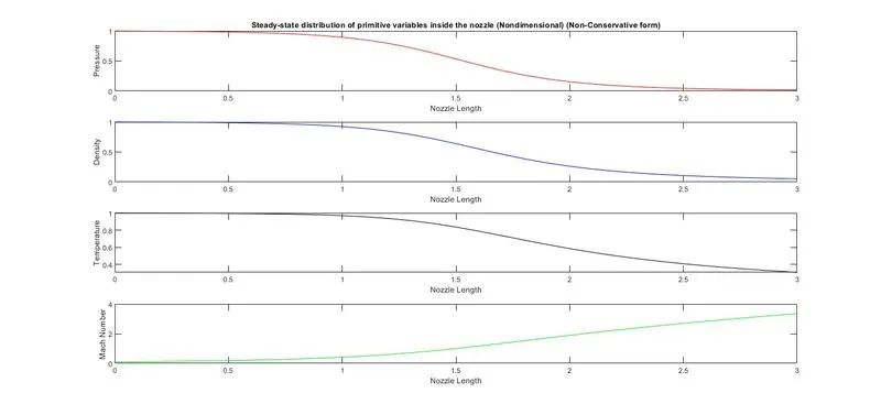
1. Steady-state distribution of primitive variables inside the nozzle
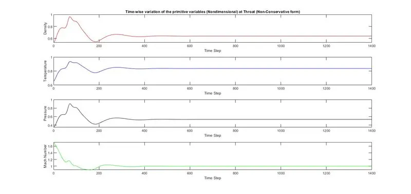
2. Time-wise variation of the primitive variables
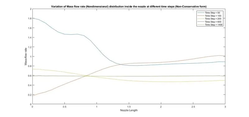
3. Variation of Mass flow rate distribution inside the nozzle at different time steps during the time-marching process.
- Conservation form (Number of nodes = 31)
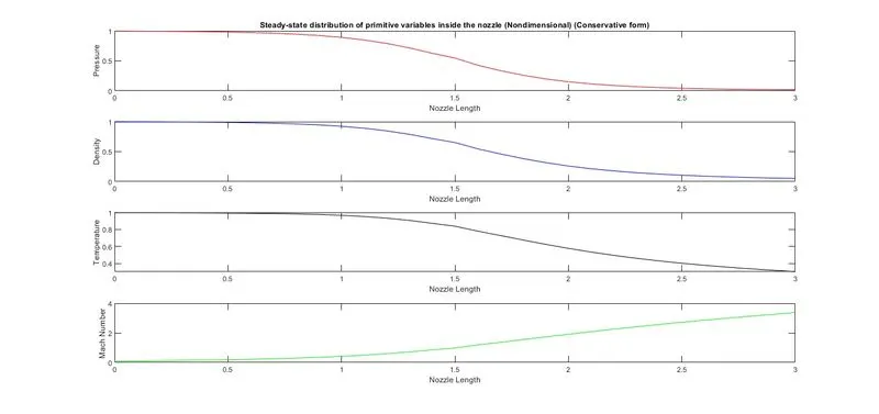
1. Steady-state distribution of primitive variables inside the nozzle
2. Time-wise variation of the primitive variables
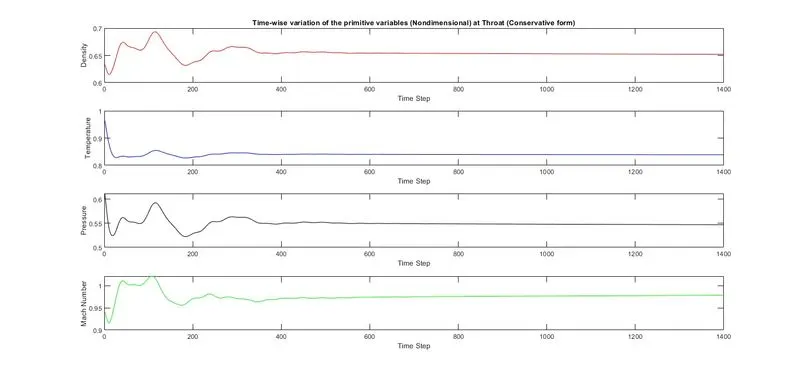
3. Variation of Mass flow rate distribution inside the nozzle at different time steps during the time-marching process.
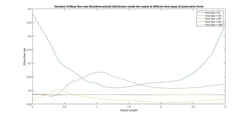
Comparison of steady state mass flow rate distributions of both forms (n = 31)
From the figures it is evident that both the non-conservative and conservative form give the same results. The usage of these method totally depend upon the available conditions, nature of problems and parameters being measured.
From the plots it can conclude that there is no clear superiority of either form in terms of accuracy of the results. The non-conservation form seems to produce slightly more accurate results for the primitive variables and the conservation form seems to produce slightly more accurate for the flux variables and yields a better mass flow distribution.
While comparing the amount of computational time and calculation conservation form requires marginally more work when compared with non-conservation form.
Grid Independence Test
| `rho^**/rho_0` | `p^**/p_0` | `T^**/T_0` | M | |
|
Non-Conservation form (n = 31) |
0.6387 | 0.5342 | 0.8365 | 0.9994 |
|
Non-Conservation form (n = 61) |
0.6377 | 0.5327 | 0.8354 | 0.9998 |
|
Non-Conservation form (n = 91) |
0.6404 | 0.5359 | 0.8368 | 1.0026 |
|
Conservation form (n = 31) |
0.6520 | 0.5470 | 0.8389 | 0.9786 |
|
Conservation form (n = 61) |
0.6388 | 0.5325 | 0.8335 | 0.9983 |
|
Conservation form (n = 91) |
0.6379 | 0.5316 | 0.8333 | 1.0007 |
| Exact Solution | 0.634 | 0.528 | 0.833 | 1 |
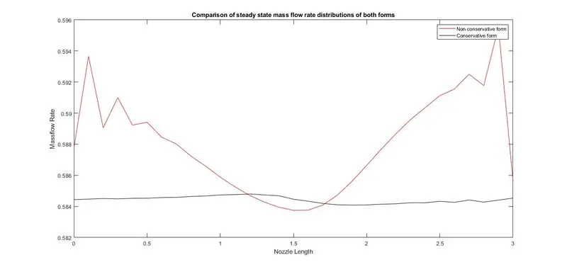
- Comparison of steady state mass flow rate distribution of both form (n = 31)
- Comparison of steady state mass flow rate distribution of both form (n = 61)
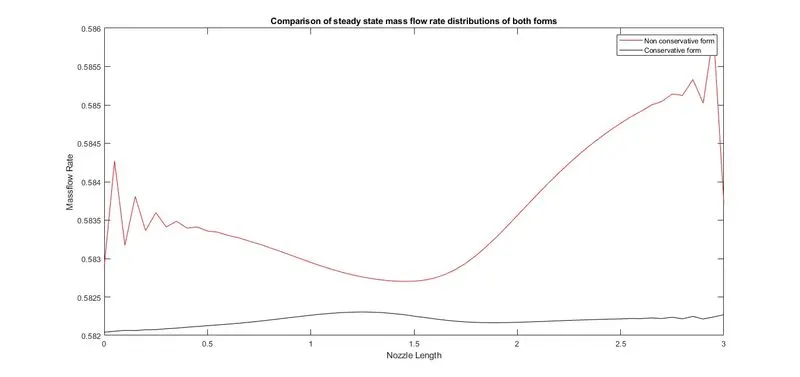
- Comparison of steady state mass flow rate distribution of both form (n = 91)
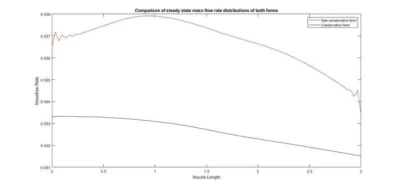
From the table of grid independence test it is evident that with increase in number of nodes from 31 to 61 the value become more close to the exact values. But with further increase to 91 the value again starts to deviate for the non-conservative form. So it can be concluded that for the non conservative form optimum grid points are 61 to get a solution more close to the exact solution. In case of conservation form with increase of grid points from 31 to 91 the values of primitive variables become more close to the exact solution thus it can be conclude that for conservation form the optimum grid points are 91 to get a solution more close to the exact solution.
It is also observed that the non-conservation form seems to produce slightly more accurate results for the primitive variables and the conservation form yields a better mass flow distribution.
CONCLUSION:
A Matlab program to simulate the isentropic flow through a quasi 1D subsonic-supersonic nozzle by both the conservation and non-conservation forms of the governing equations by using the MacCormack's technique has been created and a study is also carried out by comparing the results obtained from conservation form and non-conservation form. It is then concluded that there is no clear superiority of either form in terms of accuracy of the results and the usage of these method totally depend upon the available conditions, the nature of problems and the parameters being measured.
Reference
- Anderson Jr, John D. "Computational fluid dynamics-An engineering tool." ASME Numerical/Laboratory Computer Methods in Fluid Mechanics (1976).