Week 7 - Simulation of a 1D Super-sonic nozzle flow simulation using Macormack Method

Week 7 -

Simulation of a 1D Super-sonic nozzle flow simulation using Macormack Method

Question :

In this challenge you are going to simulate the isentropic flow through a quasi 1D subsonic-supersonic nozzle. You will derive both the conservation and non-conservation forms of the governing equations and solve them using the MacCormack's technique. You need to determine the steady-state temperature distribution for the flow-field variables and investigate the difference between the two forms of governing equations by comparing their solutions.

You need to show the following plots inside your report

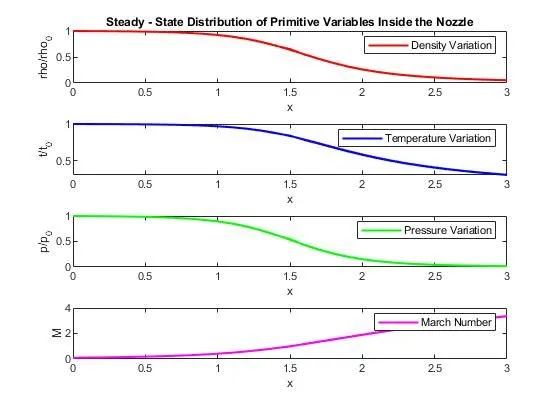
1. Steady-state distribution of primitive variables inside the nozzle
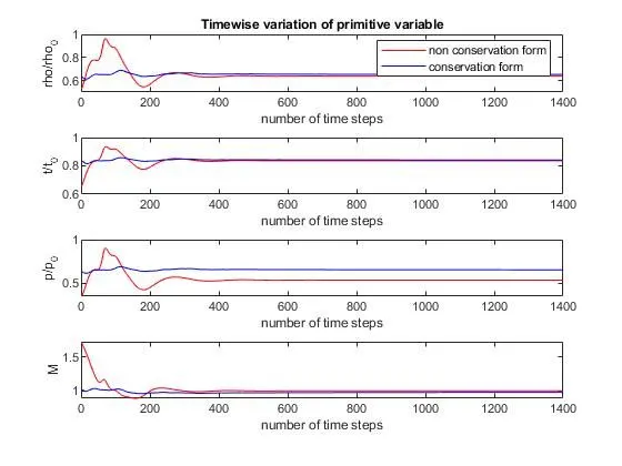
2. Time-wise variation of the primitive variables
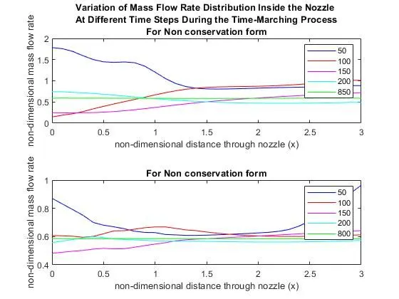
3. Variation of Mass flow rate distribution inside the nozzle at different time steps during the time-marching process
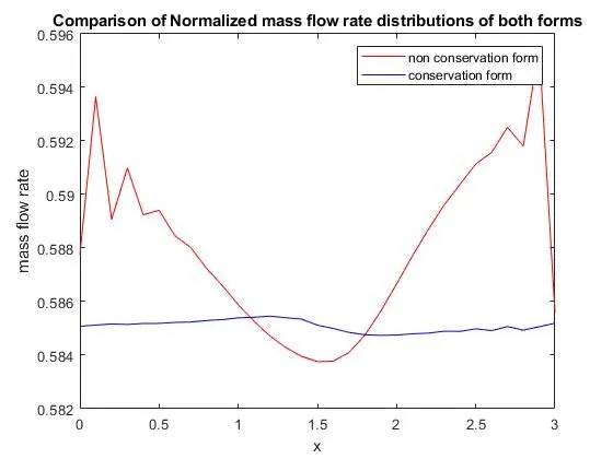
4. Comparison of Normalized mass flow rate distributions of both forms.

Expected Results:

Perform a grid independence test on the solution and expain all your findings.

The code must be modular. You need to write separate functions to solve both forms.

Discuss all the plots you are providing with observed inferences.

Aim :

To simulate the isentropic flow through a quasi 1D subsonic-supersonic nozzle using both the conservation and non-conservation forms of the governing equations and sovle them using the MacCormack's technique and comparing their solutions.

Key Points :

• Isentropic flow through a quasi 1D subsonic-supersonic nozzle
• Conservation and non-conservation forms
• The MacCormack's technique

Quasi 1D Flow :

A quasi-one-dimensional flow is one in which all variables vary primarily along one direction, say x. A flow in a duct with slowly-varying area A(x) is the case of interest here. In practice this means that the slope of the duct walls is small.

Engineers call this type of flow an isentropic flow; a combination of the Greek word "iso" (same) and entropy. Isentropic flows occur when the change in flow variables is small and gradual. The generation of sound waves is an isentropic process.

The area where the diameter is minimum is called the throat. As the gas enters the converging section, its velocity increases, considering the mass flow rate to be constant, it attains subsonic velocity (Mach number < 1).

Supersonic and subsonic flow:

Supersonic and subsonic refer to speeds faster or slower than the speed of sound. Anything going faster than the speed of sound, 343.2 m/s (1,126 ft/s), is traveling at supersonic speeds. Anything going slower than the speed of sound is traveling at subsonic speeds.

Steady ,isentropic flow through the Nozzle :

We consider steady, isentropic flow through the convergent- divergent nozzle in the fig.

The flow at the inlet of the nozzle comes from a reservoir.

At Inlet, `P_o =`and `T_o` are pressure and temperature respectively.

The cross-sectional area of the reservoir is large and hence the velocity is very small and V tends to zero. The flow expands isentropically to the supersonic speeds.

Pressure, temperature, Velocity and Mach number

The flow is locally subsonic at convergent section of the nozzle and locally supersonic at the divergent section of the nozzle.

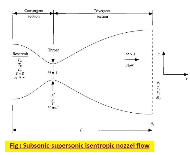
The sonic flow is M=1 at the throat, M<1 at the entrance and M>1 at the exit.

At sonic value flow V=V*=a*

Area of sonic throat A=A*

in reality the flow is in 2d but we consider only the 1d i.e in x axis so the flow is defined as Quasi 1-d flow.

Conservation and non-conservation forms of equation:

Conservation form or Eulerian form refers to an arrangement of an equation or system of equations, usually representing a hyperbolic system, that emphasizes that a property represented is conserved, i.e. a type of continuity equation. The term is usually used in the context of continuum mechanics.

The conservative form derives from expressing the conservation equations in a divergence form, i.e. the equations have the form of local time rate of change + divergence of flux = source terms. The non-conservative form is a form of the equations that is not expressible in this form. One of the principle advantages to the the conservative form is that once the equations are discretized, the flux terms "telescope", that is if you sum the fluxes into and out of a row of cells, the intercell fluxes cancel and the net flux is just the flux out of one end of the row - flux in the other end.

Governing Equations :

Non-conservative form :

Continuity Equation

`(∂ρ^')/(∂t^' )=-ρ^' (∂v^')/(∂x^' )-ρ^' v^' (∂(ln⁡A^'))/(∂x^' )-v^' (∂ρ^')/(∂x^' )`

Momentum Equation

`(∂v^')/(∂t^' )=-v^' (∂v^')/(dx^' )-1/γ ((∂T^')/(∂ϰ^1 )+(T^' ∂ρ^')/(∂x^' ))`

Energy Equation

`(∂T^')/(∂t^' )=-v (∂T^')/(∂x^' )-(γ-1) T^' [(∂v^')/(∂x^' )+v (∂(ln⁡A^'))/(∂x^' )]`

Conservative form :

Continuity Equation

`(∂(ρ^' A'))/(∂t^' )+((∂ρ^' A'v'))/(∂x^' )=0`

Momentum Equation

`(∂(ρ^' A'v'))/(∂t^' )+(∂(ρ^' A^' v^'2+(1/γ)ρ^' A^'))/(∂x^' ) = 1/γ ρ^' ((∂A^')/(∂x^' ))`

Energy Equation

`(∂(ρ^' (e^'/(γ-1)+γ/2 v^('2) ) A^' ))/(∂t^' )+(∂(ρ^' (e^'/(γ-1)+γ/2 v^('2) ) v^' A^'+ρ^' v^' A^' ))/(∂x^' )=0`

Lets express the equations for the quasi-one-dimensional flow in generic form. We're going to define the solution vector U, the flux vector F, and the source term J as follows:

`U_1=ρ^' A^'`

`U_2=ρ^' A^' v^' = U_1 v`

`U_3=ρ^' (e^'/(γ-1)+γ/2 v^2 ) A^'`

`F_1=ρ^' A^' v^'`

`F_2=ρ^' A^' v^'2+ 1/γ ρ^' A^'`

`F_3=ρ^' (e^'/(γ-1)+γ/2 v^('2) ) A^' v^'+ρ^' A^' v^'`

`J_2= 1/γ ρ^' (∂A^')/(∂x^' )`

Now , substituting these terms in above equations we get,

`(∂U_1)/(∂t^' )=-(∂F_1)/(∂x^' )`

`(∂U_2)/(∂t^' )=-(∂F_2)/(∂x^' )+ J_2`

`(∂U_3)/(∂t^' )=-(∂F_3)/(∂x^' )`

The initial and boundary conditions are calculated as follows.

Initial Conditions :

The nozzle's shape, A = A(x), is specified and held fixed, independent of time. For the case illustrated in this section, we're choosing a parabolic area distribution given by:

`A=1+2.2(x-1.5)^2 where, x is 0 ≤ x ≤ 3`

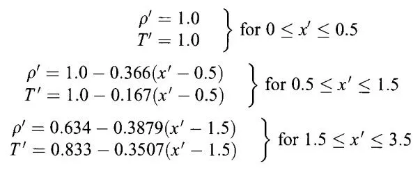
Dependent variables which are being solved from the governing equations are U1, U2 & U3. We need initial conditions for these same variables at time t = 0 in order to start the finite-difference solution. The initial conditions for U1, U2, and U3 will also allow initial conditions for F1, F2 & F3 to be obtained from the above equations. Such initial conditions for F1, F2 & F3 are needed to form the x derivatives on the right-hand sides of the governing equations at the first time step.

The initial conditions for U1, U2, and U3 were synthesized by assuming the following variations

Boundary Conditions:

Boundary conditions are important because the applicability of numerical methods and the resultant quality of computations can critically be decided on how those are numerically treated and without the proper implementation of boundary conditions and their numerically proper representation, we have no hope whatsoever of obtaining a proper numerical solution to our flow problem.

Many important problems such as flow driven by moving objects, free-surface flow, flow involving air bubbles, flow accompanying phase transition, and fluid-structure interaction, are moving boundary problems. In dealing with such boundaries with movement or deformation, the traditional mesh methods such as finite difference method, finite element method, and finite volume method generally encounter difficulties in calculating accurately the geometric shape of the boundary.

Need of Boundary condition:

• It is necessity to solve Navier Stoke(NS) equations.
• Geometry and operating conditions are the only 2 inputs to NSE that are unique from problem to problem.

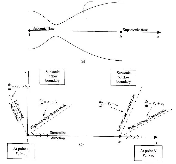
SUBSONIC INFLOW BOUNDARY CONDITIONS AT POINT 1:

At the subsonic inflow boundary, two properties are held fixed and one is allowed to float & at the supersonic outflow boundary all properties are allowed to float. In the present formulation, just as before, we're holding pressure and temperature fixed at the inflow boundary, both equal to 1.0 and it allows V’ to float. By holding p’

fixed, then the U1 at grid point i =1 is fixed independent to time, via `U_1 = rho'A'`

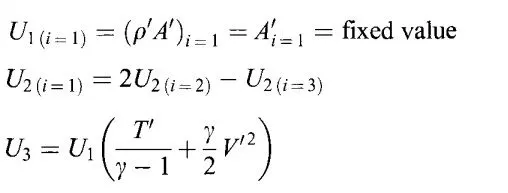
SUPERSONIC OUTFLOW BOUNDARY AT POINT N:

In the case of the supersonic outflow boundary, all properties are allowed to float. The flow properties at the downstream, supersonic outflow boundary are obtained by linear extrapolation from the two adjacent internal points. If N denotes the grid point at the outflow boundary, then:

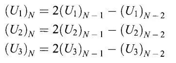
Discretizing the domain :

Domain is discretized to N nodes with 1 node indicating the reservoir where the inflow boundary conditions is specified and the node N is used for the outflow boundary conditions.

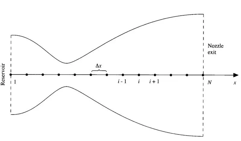
MacCormack technique :

The MacCormack method is a widely used discretization scheme for the numerical solution of hyperbolic partial differential equations. This second-order finite difference method was introduced by Robert W. MacCormack in 1969. The MacCormack method is elegant and easy to understand and program.

The MacCormack method is a variation of the two-step Lax–Wendroff scheme but is much simpler in application.

The MacCormack method is well suited for nonlinear equations (Inviscid Burgers equation, Euler equations, etc.) The order of differencing can be reversed for the time step (i.e., forward/backward followed by backward/forward). For nonlinear equations, this procedure provides the best results. For linear equations, the MacCormack scheme is equivalent to the Lax–Wendroff method.

Unlike first-order upwind scheme, the MacCormack does not introduce diffusive errors in the solution. However, it is known to introduce dispersive errors (Gibbs phenomenon) in the region where the gradient is high.

Its a two step procedure: predictor step and corrector step

Predictor step:

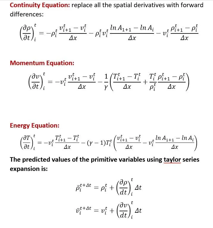
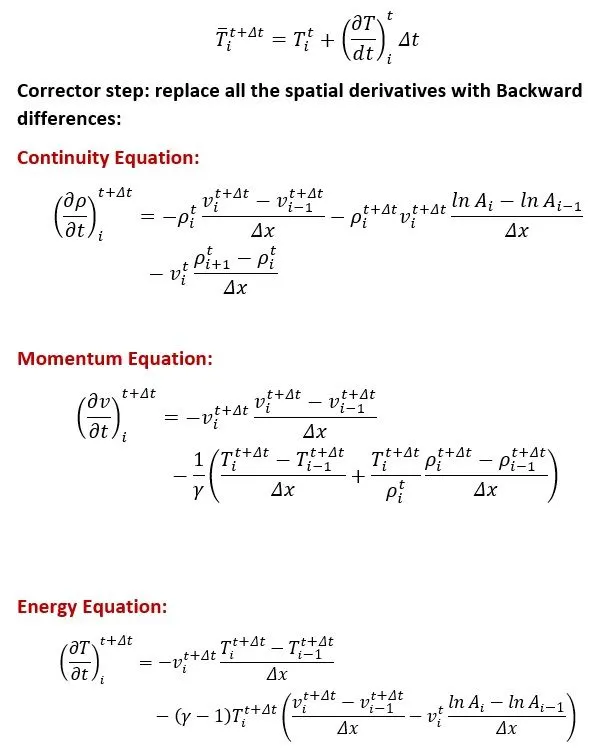
Finding the average value of derivative : This term is actually providing us the second order accuracy

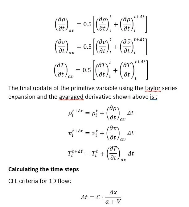
C is the courant number, which must satisfy C≤1 (since governing equations are hyperbolic with respect to time), this simply indicates Δt ≤ the time required for the sound wave to move from one grid point to the next.

V=local flow velocity and a=local speed of sound. Although

Δx is constant both V and vary throughout the flow. hence in order to implement time marching, we can use the following two methods:

local time-stepping:

the different time step is calculated at each of the grid points

not accurate for unsteady flow.

this method is useful and gives faster convergence when the only final steady-state analysis is desired and intermediate variations are irrelevant.

MATLAB CODE:

Programming Language: MATLAB

Main Program of Nozzle flow

clear
close 
clc

%% Inputs
n=31; % Number of grid points
L=3; % Length of nozzle
throat=(n+1)/2; %Throat- Least area
x=linspace(0,L,n); % Defining Mesh
dx=x(2)-x(1); %Grid Spacing
gamma=1.4; %Ratio of specific heat
C=0.5; %Courant Number

%time steps 
nt=1400;
dt=0.0204; 

% nonconservative form
[rho_nc,v_nc,t_nc,M_nc,p_nc,rho_nc_t,t_nc_t,p_nc_t,M_nc_t,m_nc]=nonc(gamma,dx,nt,dt,n,x,throat);

%conservative form
[rho_c,v_c,t_c,p_c,M_c,rho_c_t,t_c_t,p_c_t,M_c_t,m_c]=conv(gamma,dx,x,n,nt,dt,throat);

%% plotting the results
% steady state results
% steady-state variations of the primitive variable (rho,t, M,p) along the length of the nozzle (x)
figure(1)
subplot(4,1,1)
plot(x,rho_nc,x,rho_c,'Color','r','LineWidth',1.5);
legend('Density Variation');
xlabel('x')
ylabel('rho/rho_0');
title('Steady - State Distribution of Primitive Variables Inside the Nozzle');


subplot(4,1,2)
plot(x,t_nc,x,t_c,'Color','b','LineWidth',1.5);
legend('Temperature Variation');
xlabel('x')
ylabel('t/t_0');

subplot(4,1,3)
plot(x,p_nc,x,p_c,'Color','g','LineWidth',1.5);
legend('Pressure Variation');
xlabel('x')
ylabel('p/p_0');

subplot(4,1,4)
plot(x,M_nc,x,M_c,'Color','m','LineWidth',1.5);
legend('March Number');
xlabel('x')
ylabel('M');



%timewise variation of primitive variable
%variation of primitive variables (rho,t,M,andp) with respect to timesteps
%for both conservation and non-conservation forms at the throat section
figure(2)
subplot(4,1,1);
plot(1:nt,rho_nc_t,'r-',1:nt,rho_c_t,'b');
legend('non conservation form','conservation form');
xlabel('number of time steps')
ylabel('rho/rho_0');
title('Timewise variation of primitive variable')

subplot(4,1,2);
plot(1:nt,t_nc_t,'r-',1:nt,t_c_t,'b');
xlabel('number of time steps')
ylabel('t/t_0');

subplot(4,1,3);
plot(1:nt,p_nc_t,'r-',1:nt,p_c_t,'b');
xlabel('number of time steps')
ylabel('p/p_0');

subplot(4,1,4);
plot(1:nt,M_nc_t,'r-',1:nt,M_c_t,'b');
xlabel('number of time steps')
ylabel('M');

%comparison of the variation of mass flow rate in both the forms
figure(3)
plot(x,m_nc,'r-',x,m_c,'b');
legend('non conservation form','conservation form');
xlabel('x')
ylabel('mass flow rate');
title('Comparison of Normalized mass flow rate distributions of both forms')

Function for Non-conservative form

function [rho,v,t,M,p,rho_nc_t,t_nc_t,p_nc_t,M_nc_t,m]=nonc(gamma,dx,nt,dt,n,x,throat);

%initial profiles
rho=1-0.3146*x; %Density
t=1-0.2314*x; %Temperature
v=(0.1+1.09*x).*t.^0.5; %Velocity
a=1+2.2*(x-1.5).^2; %Area

for k=1:nt %Outer time loop
    % Old variables
    rho_old=rho;
    v_old=v;
    t_old=t;
    %predictor method
    for j=2:n-1
        %Forward Differencing
        dvdx=(v(j+1)-v(j))/dx;
        drhodx=(rho(j+1)-rho(j))/dx;
        dtdx=(t(j+1)-t(j))/dx;
        dlog_a_dx=(log(a(j+1))-log(a(j)))/dx;
        
        %continuity equation
        drhodt_p(j)=-rho(j).*dvdx-rho(j).*v(j)*dlog_a_dx-v(j).*drhodx;
        
        %momentum equation
        dvdt_p(j) =-v(j).*dvdx-(1/gamma).*(dtdx+(t(j)/rho(j)).*drhodx);
        
        %energy equation
        dtdt_p(j)=-v(j).*dtdx-(gamma-1).*t(j).*(dvdx+(v(j).*dlog_a_dx));
        
        
        %solution update
        rho(j)=rho(j)+drhodt_p(j)*dt;
        v(j)=v(j)+dvdt_p(j)*dt;
        t(j)=t(j)+dtdt_p(j)*dt;
    end
    
    %corrector method
    for j=2:n-1 % For inner nodes
        % Backward Differencing
        dvdx=(v(j)-v(j-1))/dx;
        drhodx=(rho(j)-rho(j-1))/dx;
        dtdx=(t(j)-t(j-1))/dx;
        dlog_a_dx=(log(a(j))-log(a(j-1)))/dx;
        
        %continuity
        drhodt_c(j)=-rho(j).*dvdx-rho(j).*v(j)*dlog_a_dx-v(j).*drhodx;
        
        %momentum equation
        dvdt_c(j) =-v(j).*dvdx-(1/gamma).*(dtdx+(t(j)/rho(j)).*drhodx);
        
        %energy equation
        dtdt_c(j)=-v(j).*dtdx-(gamma-1).*t(j).*(dvdx+(v(j).*dlog_a_dx));
    end
        
    %compute average time derivative
    drhodt=0.5*(drhodt_p+drhodt_c);
    dvdt=0.5*(dvdt_p+dvdt_c);
    dtdt=0.5*(dtdt_p+dtdt_c);
       
    %final solution update
    for i=2:n-1
        rho(i)=rho_old(i)+drhodt(i)*dt;
        v(i)=v_old(i)+dvdt(i)*dt;
        t(i)=t_old(i)+dtdt(i)*dt;
    end
    
    %apply boundary conditions
    %At inlet
    v(1)=2*v(2)-v(3);
    %At outlet
    rho(n)=2*rho(n-1)-rho(n-2);
    v(n)=2*v(n-1)-v(n-2);
    t(n)=2*t(n-1)-t(n-2);
    
 
    %defining other flow field variables
    
    M=v./(t.^0.5); %March number
    p=rho.*t; %Pressure
    m=rho.*a.*v; %Mass flow rate
    %mass flow rate w.r.t initial conditions
    m_0t=rho_old.*a.*v_old;
    
    %storing values of primitive variables at throat w.r.t to time steps
    rho_nc_t(k)=rho(throat);
    M_nc_t (k)=v(throat)./(t(throat).^0.5);
    p_nc_t (k)=rho(throat).*t(throat);
    t_nc_t(k)=t(throat);
    
    %Instantaneous distribution of nondimensional mass flow 
    %as a function of distance through the nozzle at five different times 
    %during the time marching approach to the steady state
    
        figure(4)
    subplot(2,1,1);
    if k==50
        plot(x,m,'b');
        hold on
    elseif k==100
        plot(x,m,'r');
    elseif k==150
        plot(x,m,'m');
    elseif k==200
        plot(x,m,'c');
    elseif k==850
        plot(x,m,'g');
    
xlabel('non-dimensional distance through nozzle (x)');
ylabel('non-dimensional mass flow rate');
legend('50','100','150','200','850');
title(sprintf('Variation of Mass Flow Rate Distribution Inside the Nozzle \n At Different Time Steps During the Time-Marching Process \n For Non conservation form '));
end
end

Function for Conservative form

function [rho,v,t,p,M,rho_c_t,t_c_t,p_c_t,M_c_t,m]=conv(gamma,dx,x,n,nt,dt,throat);

%initial profiles
for i=1:n
    if (x(i)<0.5)
        rho(i)=1;
        t(i)=1;
    elseif (x(i)>=0.5 && (x(i)<=1.5))
        rho(i)=1-(0.366*(x(i)-0.5));
        t(i)=1-(0.167*(x(i)-0.5));
    else
        rho(i)=0.634-(0.3879*(x(i)-1.5));
        t(i)=0.833-(0.3507*(x(i)-1.5));
    end
end

a=1+2.2*(x-1.5).^2;
v=0.59./(rho.*a);
u1=rho.*a;
u2=rho.*a.*v;
u3=u1.*((t./(gamma-1))+((gamma/2).*(v.^2)));
    
for k=1:nt
    u1_old=u1; %i=31 only copies the last element of u1,u2 and u3
    u2_old=u2;
    u3_old=u3;
    
    %flux 
    f1=u2;
    f2=((u2.^2)./u1)+(((gamma-1)/gamma).*(u3-((gamma/2)*((u2.^2)./u1))));
    f3=(((gamma.*u2.*u3)./u1)-(gamma.*((gamma-1)/2).*((u2.^3)./(u1.^2))));
    
    %predictor step
    for j=2:n-1
      
     du1dt_p(j)=-(f1(j+1)-f1(j))/dx;
     j2(j)=(1/gamma)*rho(j)*t(j)*((a(j+1)-a(j))/dx);
     du2dt_p(j)=-(f2(j+1)-f2(j))/dx+j2(j);
     du3dt_p(j)=-(f3(j+1)-f3(j))/dx;
     
     %solution update
     u1(j)=u1(j)+du1dt_p(j)*dt;
     u2(j)=u2(j)+du2dt_p(j)*dt;
     u3(j)=u3(j)+du3dt_p(j)*dt;

  end
    %primitive variables update
     rho=u1./a;
     v=u2./u1;
     t=(gamma-1).*((u3./u1)-((gamma/2).*(v.^2)));
    %flux update for corrector
    f1=u2;
    f2=((u2.^2)./u1)+(((gamma-1)/gamma).*(u3-((gamma/2)*((u2.^2)./u1))));
    f3=(((gamma.*u2.*u3)./u1)-(gamma.*((gamma-1)/2).*((u2.^3)./(u1.^2))));
    %corrector method
    for j=2:n-1
        
        df1dx=((f1(j)-f1(j-1))/dx);
        df2dx=((f2(j)-f2(j-1))/dx);
        df3dx=((f3(j)-f3(j-1))/dx);
        
        %continuity
        du1dt_c(j)=-df1dx;
        j2(j)=(1/gamma)*rho(j)*t(j)*((a(j)-a(j-1))/dx); %j2 has to be recalculated with backward difference
        %momentum equation
        du2dt_c(j)=-df2dx+j2(j);
        
        %energy equation
        du3dt_c(j)=-df3dx; %No j2 for du3dt
    end
        
    %compute average time derivative
    du1dt=0.5*(du1dt_p+du1dt_c);
    du2dt=0.5*(du2dt_p+du2dt_c);
    du3dt=0.5*(du3dt_p+du3dt_c);
       
    %final solution 
    for i=2:n-1
        u1(i)=u1_old(i)+du1dt(i)*dt;
        u2(i)=u2_old(i)+du2dt(i)*dt;
        u3(i)=u3_old(i)+du3dt(i)*dt;
    end
    %apply boundary conditions
    %inlet
    u2(1)=2*u2(2)-u2(3);
    v(1)=u2(1)/u1(1);
    u3(1)=u1(1)*((t(1)/(gamma-1))+(0.5*gamma*v(1)^2));
    %outlet
    u1(n)=2*u1(n-1)-u1(n-2);
    u2(n)=2*u2(n-1)-u2(n-2);
    u3(n)=2*u3(n-1)-u3(n-2);    
    
     %Final primitive variables update 
     rho=u1./a;
     v=u2./u1;
     t=(gamma-1).*((u3./u1)-((gamma/2).*(v.^2)));
     
   %defining othe flow field variables
    M=v./(t.^0.5);
    p=rho.*t;
    m=rho.*a.*v;
    
    %storing values of primitive variables at throat w.r.t to time steps
    rho_c_t(k)=rho(throat);
    t_c_t(k)=t(throat);
    p_c_t(k)=rho(throat);
    M_c_t(k)=M(throat);
    
    %Instantaneous distribution of nondimensional mass flow 
    figure(4)
    subplot(2,1,2);
    if k==50
        plot(x,m,'b');
        hold on
    elseif k==100
        plot(x,m,'r');
    elseif k==150
        plot(x,m,'m');
    elseif k==200
        plot(x,m,'c');
    elseif k==800
        plot(x,m,'g');
    xlabel('non-dimensional distance through nozzle (x)');
    ylabel('non-dimensional mass flow rate');
    legend('50','100','150','200','800')
title('For Non conservation form');
end
end

Output Plots :

Conclusion:

• The steady-state variation of primitive variables along the length x for both conservation and non-conservation forms show exact same variations
• The density, temperature, and pressure decrease as the flow proceeds along the length of the nozzle.
• The Mach no. is <1 (subsonic) at nozzle entry, =1 at throat and >1 (supersonic) at nozzle exit.

• The timewise variation of the primitive variables with respect to the number of time steps for both conservation and non-conservation forms denotes that the variations are large at smaller time steps, the changes in the flow field variables reduce at a larger value of time steps when the solution approaches a steady state.
• It can also be observed that initial variations in the case of conservation form are much lesser compared to that of non-conservation form which is probably due to a more improved definition of the initial condition in the case of the former.

• We can observe from the variation of the mass flow rate along the length of the nozzle at different time steps for both conservation and non-conservation forms.
• The different curves represent a variation of mass flow after 50,100, 150, 200, and 850-time steps for the non-conservation form, and the last timestep for conservation form is 800.
• It is observed the variation changes drastically after these time steps, slowly approaching towards a constant value at the 850th time step in case of non-conservation form and at 8000 at conservation form. This indicates that the mass flow rate is converged to a constant, steady-state value throughout the nozzle.

• Comparison of the normalized mass flow rate distribution between both forms suggests that the conservation form preserves the mass flow rate throughout the flow field in a better manner than the non-conservation form.
• This is because the mass flow rate is a primary result of these equations (U2=rho*A*V). while in case of non-conservation form the mass flow rate is obtained as a secondary result
• As the conservation form does a better job of conserving the mass flow rate we can understand why they are called conservation form.

GRID INDEPENDENCE TEST :

The grid independence test is a process used to find the optimal grid condition that has the smallest number of grids without generating a difference in the numerical results based on the evaluation of various grid conditions.

Here, we are going to conduct a grid independence test on the 1-D subsonic – supersonic nozzle flow problem by increasing the number of grid points from 31 to 61.

we can observe that, even with the increase in the number of grid points, there is no effect on the primitive variable values for both the conservative and non- conservative forms. We can also observe that, with the increase in the number of grid points, the numerical solution values are much closer to the analytical or real solution of the equation, when compared to that of the lesser number of grid points. Therefore, we can clearly say that the 1-D subsonic – supersonic problem is grid independent.

Reference:

• http://mae-nas.eng.usu.edu/MAE_5420_Web/section4/section4.1.pdf
• http://web.mit.edu/16.unified/www/SPRING/fluids/Spring2008/LectureNotes/f19.pdf
• https://www.grc.nasa.gov/WWW/K-12/airplane/isentrop.html
• https://ui.adsabs.harvard.edu/abs/2017ExFl...58...64L/abstract
• https://featips.com/2019/03/31/what-is-a-mesh-independence-study/