Week 7 - Simulation of a 1D Super-sonic nozzle flow simulation using Macormack Method
Program:
clear all;
close all;
clc;


tic;
nx_nc = 31;        %No. of nodes
l_nc = 3;          %Length of the domain
x_nc = linspace(0,l_nc,nx_nc);   %Mesh generation
dx_nc = l_nc/(nx_nc-1);

t_nc = 1400;  %time
A_throat_nc = 1;
gamma_nc = 1.4;
C_nc = 0.2;       % Courant Number

%Initial conditions based on shape of the nozzle
A_nc = 1+2.2*(x_nc-1.5).^2;
rho_nc = 1-0.3146*x_nc;
T_nc = 1-0.2314*x_nc;
V_nc = (0.1+1.09*x_nc).*T_nc.^0.5;


for k = 1:t_nc        %time marching
    rho_old_nc = rho_nc;
    V_old_nc = V_nc;
    T_old_nc = T_nc;
    A_old_nc = A_nc;

    dt_nc = C_nc*dx_nc./((T_nc.^0.5)+V_nc);     %Courant number criterion
    dt_nc = min(dt_nc);              % taking time step as minimun value after calculating at each node
    for i = 2: nx_nc-1     %space marching

        % predictor step , forward differencing of space terms
        dV_dx_nc = (V_nc(i+1)-V_nc(i))/dx_nc;
        dlogA_dx_nc = (log(A_nc(i+1))-log(A_nc(i)))/dx_nc;
        drho_dx_nc = (rho_nc(i+1)-rho_nc(i))/dx_nc;
        dT_dx_nc = (T_nc(i+1)-T_nc(i))/dx_nc;

        drho_dt_p_nc(i) = -rho_nc(i)*(dV_dx_nc)-(rho_nc(i).*V_nc(i)*dlogA_dx_nc)-(V_nc(i)*drho_dx_nc);
        dV_dt_p_nc(i) = (-V_nc(i)*dV_dx_nc)-((1/gamma_nc)*(dT_dx_nc+(T_nc(i)/rho_nc(i))*drho_dx_nc));
        dT_dt_p_nc(i) = -V_nc(i)*(dT_dx_nc)-(gamma_nc-1)*T_nc(i)*(dV_dx_nc+(V_nc(i)*dlogA_dx_nc));


        %Solution update
        rho_nc(i) = rho_old_nc(i) + drho_dt_p_nc(i)*dt_nc;
        V_nc(i) = V_old_nc(i) + dV_dt_p_nc(i)*dt_nc;
        T_nc(i) = T_old_nc(i) + dT_dt_p_nc(i)*dt_nc;

    end

    for i = 2: nx_nc-1     %space marching

        % corrector step , backward differencing of space terms
        dV_dx_nc = (V_nc(i)-V_nc(i-1))/dx_nc;
        dlogA_dx_nc = (log(A_nc(i))-log(A_nc(i-1)))/dx_nc;
        drho_dx_nc = (rho_nc(i)-rho_nc(i-1))/dx_nc;
        dT_dx_nc = (T_nc(i)-T_nc(i-1))/dx_nc;

        drho_dt_c_nc(i) = -rho_nc(i)*(dV_dx_nc)-(rho_nc(i).*V_nc(i)*dlogA_dx_nc)-(V_nc(i)*drho_dx_nc);
        dV_dt_c_nc(i) = (-V_nc(i)*dV_dx_nc)-((1/gamma_nc)*(dT_dx_nc+(T_nc(i)/rho_nc(i))*drho_dx_nc));
        dT_dt_c_nc(i) = -V_nc(i)*(dT_dx_nc)-(gamma_nc-1)*T_nc(i)*(dV_dx_nc+(V_nc(i)*dlogA_dx_nc));

    end
    %computing the average
    drho_dt_avg_nc = 0.5*(drho_dt_p_nc + drho_dt_c_nc);
    dV_dt_avg_nc = 0.5*(dV_dt_p_nc + dV_dt_c_nc);
    dT_dt_avg_nc = 0.5*(dT_dt_p_nc + dT_dt_c_nc);

    %final solution update

    for i = 2:nx_nc-1
        rho_nc(i) = rho_old_nc(i) + drho_dt_avg_nc(i)*dt_nc;
        V_nc(i) = V_old_nc(i) + dV_dt_avg_nc(i)*dt_nc;
        T_nc(i) = T_old_nc(i) + dT_dt_avg_nc(i)*dt_nc;
    end

    %boundary conditions

    %Boundary condition at node-1(Reservior)
    V_nc(1) = 2*V_nc(2)-V_nc(3);
    rho_nc(1) = 1;
    T_nc(1) = 1;
    %Boundary condition at end node(outlet)
    V_nc(nx_nc) = 2*V_nc(nx_nc-1)-V_nc(nx_nc-2);
    rho_nc(nx_nc) = 2*rho_nc(nx_nc-1)-rho_nc(nx_nc-2);
    T_nc(nx_nc) = 2*T_nc(nx_nc-1)-T_nc(nx_nc-2);

    % Calculating solutions
    % Mass flow rate
    m_nc = rho_nc.*A_nc.*V_nc;
    % pressure
    P_nc = rho_nc.*T_nc;
    % Mach number
    M_nc = V_nc./((T_nc).^0.5);

    %Non-conservative solution plot

    figure(1)
    subplot(2,3,1)
    plot(x_nc,P_nc)
    xlabel('Length of domain')
    ylabel('Pressure ratio : P/P_0')
    title('Pressure ratio V/S length of domain')

    subplot(2,3,2)
    plot(x_nc,rho_nc)
    xlabel('Length of domain')
    ylabel('Density ratio : rho/rho_0')
    title('Density ratio V/S length of domain')


    subplot(2,3,3)
    plot(x_nc,T_nc)
    xlabel('Length of domain')
    ylabel('Temperature ratio : T/T_0')
    title('Temp. ratio V/S length of domain')


    subplot(2,3,4)
    plot(x_nc,M_nc)
    xlabel('Length of domain')
    ylabel('Mach Number : M')
    title('Mach Number V/S length of domain')


    subplot(2,3,5)
    plot(x_nc,m_nc)
    xlabel('Length of domain')
    ylabel('Mass flow rate')
    title('mass flow rate V/S length of domain')
    pause(0.003)

    sgtitle(sprintf('Time step %d',k))


end
simulation_time_nc = toc;

tic;
%Conservative
gamma = 1.4;
C = 0.8;
l = 3;
nx = 31;
x = linspace(0,3,nx);
A = 1+2.2*(x-1.5).^2;
t = 1400;
dx = x(2) - x(1);

for i = 1:nx
    if x(i)>=0 && x(i)<=0.5
        rho(i) = 1;
        T(i) = 1;
    else if x(i)>=0.5 && x(i)<=1.5
            rho(i)= 1-0.366*(x(i)-0.5);
            T(i) = 1-0.167*(x(i)-0.5);
    else if x(i)>=1.5 && x(i)<=3
            rho(i) = 0.634-0.3879*(x(i)-1.5);
            T(i) = 0.833-0.3507*(x(i)-1.5);
    end
    end
    end
end
V = 0.59./(rho.*A);
P = rho.*T;
U1 = rho.*A;
U2 = rho.*A.*V;
U3 = rho.*((T./(gamma-1))+((gamma/2).*(V.^2))).*A;
dt = C*dx./((T.^0.5)+V);     %Courant number criterion
dt = min(dt);              % taking time step as minimum value after calculating at each node

for k = 1:t
    U1_old = U1;
    U2_old = U2;
    U3_old = U3;

    %Flux variables
    F1 = U2;
    F2 = ((U2.^2)./U1) + ((gamma-1)/gamma)*(U3-(((gamma/2)*U2.^2)./U1));
    F3 = ((gamma*U2.*U3)./U1) - (gamma*(gamma-1)/2)*((U2.^3)./(U1.^2));

    % predictor step , forward differencing of space terms
    for j = 2:nx-1
        dF1_dx = (F1(j+1)-F1(j))/dx;
        dF2_dx = (F2(j+1)-F2(j))/dx;
        dF3_dx = (F3(j+1)-F3(j))/dx;
        dlogA_dx = (log(A(j+1))-log(A(j)))/dx;
        dA_dx = (A(j+1)-A(j))/dx;
        J2 = (1/gamma).*rho(j).*T(j).*dA_dx;

        % continuity equation
        dU1_dt_p(j) = -dF1_dx;
        % Momentum equation
        dU2_dt_p(j) = -dF2_dx + J2;
        % Energy equation
        dU3_dt_p(j) = -dF3_dx;

        % Solution update
        U1(j) = U1(j) + dU1_dt_p(j)*dt;
        U2(j) = U2(j) + dU2_dt_p(j)*dt;
        U3(j) = U3(j) + dU3_dt_p(j)*dt;

    end

    % Primitive terms for corrector step
    rho = U1./A;
    v = U2./U1;
    t = (gamma-1)*((U3./U1)-((gamma/2)*((U2./U1).^2)));
    P = rho.*t;
    F1 = U2;
    F2 = ((U2.^2)./U1) + ((gamma-1)/gamma)*(U3-(((gamma/2)*U2.^2)./U1));
    F3 = ((gamma*U2.*U3)./U1)-(gamma*(gamma-1)/2)*((U2.^3)./(U1.^2));

    % corrector step, backward differencing of space terms
    for j=2:nx-1
        dF1_dx = (F1(j)-F1(j-1))/dx;
        dF2_dx = (F2(j)-F2(j-1))/dx;
        dF3_dx = (F3(j)-F3(j-1))/dx;
        dlogAdx = (log(A(j))-log(A(j-1)))/dx;
        dA_dx = (A(j)-A(j-1))/dx;
        J2 = (1/gamma).*rho(j).*t(j).*dA_dx;

        % continuity equation
        dU1_dt_c(j) = -dF1_dx;
        % Momentum equation
        dU2_dt_c(j) = -dF2_dx + J2;
        % Energy equation
        dU3_dt_c(j) = -dF3_dx;
    end
    % Average derivatives
    dU1_dt = 0.5*(dU1_dt_p + dU1_dt_c);
    dU2_dt = 0.5*(dU2_dt_p + dU2_dt_c);
    dU3_dt = 0.5*(dU3_dt_p + dU3_dt_c);

    % Final solution update
    for i = 2:nx-1
        U1(i) = U1_old(i) + dU1_dt(i)*dt;
        U2(i) = U2_old(i) + dU2_dt(i)*dt;
        U3(i) = U3_old(i) + dU3_dt(i)*dt;
    end
    % Applying the Boundary conditions
    % Inlet
    U1(1)=rho(1)*A(1);
    U2(1)= 2*U2(2)-U2(3);
    v(1)= U2(1)/U1(1);
    t(1) = 1;
    U3(1) = U1(1)*((t(1)/(gamma-1))+((gamma/2)*(v(1)^2)));

    % caculating solutions
    % Mass flow rate
    m = rho.*V.*A;
    % pressure
    P = rho.*t;
    % Mach number
    M= V./((T).^0.5);

    % Conservative solution plot

    figure(2)
    subplot(2,3,1)
    plot(x,P)
    xlabel('Length of domain')
    ylabel('Pressure ratio : P/P_0')
    title('Pressure ratio V/S length of domain')


    subplot(2,3,2)
    plot(x,rho)
    xlabel('Length of domain')
    ylabel('Density ratio : rho/rho_0')
    title('Density ratio V/S length of domain')


    subplot(2,3,3)
    plot(x,T)
    xlabel('Length of domain')
    ylabel('Temperature ratio : T/T_0')
    title('Temp. ratio V/S length of domain')


    subplot(2,3,4)
    plot(x,M)
    xlabel('Length of domain')
    ylabel('Mach Number : M')
    title('Mach Number V/S length of domain')


    subplot(2,3,5)
    plot(x,m)
    xlabel('Length of domain')
    ylabel('Mass flow rate')
    title('mass flow rate V/S length of domain')
    pause(0.003)

    sgtitle(sprintf('Time step %d',k))


end
simulation_time_c = toc;

%comparison plots

figure(3)
plot(x_nc,m_nc)
hold on
plot(x,m)
xlabel('Length of domain')
ylabel('Mass flow rate')
legend('non_conservative mass flow','Conservative mass flow')
title('mass flow rate V/S length of domain')

figure(4)
X = categorical({'Simulation time (Non-Conservative)','Simulation time (Conservative)'});
Y = [simulation_time_nc,simulation_time_c];
bar(X,Y)
Code Explanation
1. Code started with close all, clear all & clc command.
2. tic & toc commands are used for both non-conservative & conservative equations to keep the track of simulation time.
3. Variable having 'nc' in its name belong to the non-conservative flow field.
4. Now certain terms are defined like No. of nodes, length of domain, total time, area of throat, gamma , and Courant number.
5. Initial conditions are specified containing governing equations of area, density, temperature & velocity based on shape of the nozzle.
6. Time & space marching loop is initiated and copy of variables are made ( rho, Temp, vel).
7. The Courant number criterion for the time step is stated in which 'dt' is taken minimum of the value calculated at each node at a given time.
8. Now MacCormack method is used to calculate the final solution for continuity, momentum, and energy equations.
9. Steps in MacCormack's method are as follows-
a) Predicter step: calculated by forward differencing of differential equations.
b) Solution update
c) corrector step: calculated by backward differencing of differential equations.
d) Solution update
e) Taking the average of both predictor & corrector.
f) Final solution update.
10. Boundary conditions are defined.
a) At inlet: velocity is calculated by interpolation , rho = 1 , T =1
b) At outlet: V, rho, T all are interpolated.
11. The governing equations for mass flow rate, pressure, Mach No. are written.
12. 5 subplots are created in a single figure showing the graphs.
13. Similarly the continuity, momentum & energy equations are solved for the conservative flow field.
14. For comparison, a figure is plotted showing the mass flow rate of conservative & non-conservative flow fields.
15. A bar graph is plotted showing the simulation time of both the flow fields.
Graphs
1) Non- Conservative plot
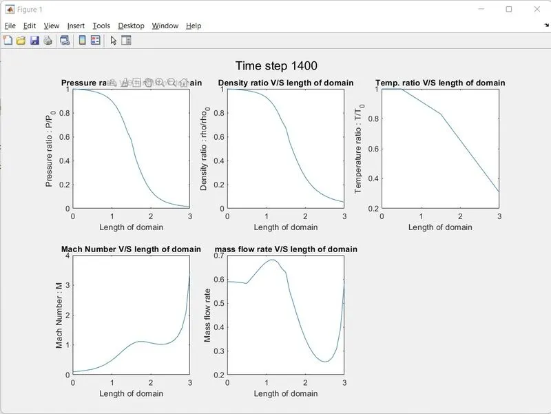
> Pressure ratio, density ratio & temperature ratio decrease along the length of the nozzle.
> Mach No. increases along the length of the nozzle & Mach No = 1 at the throat section.
> Mass flow rate is more in the convergent region as compared to the divergent region.
2) Conservative plot
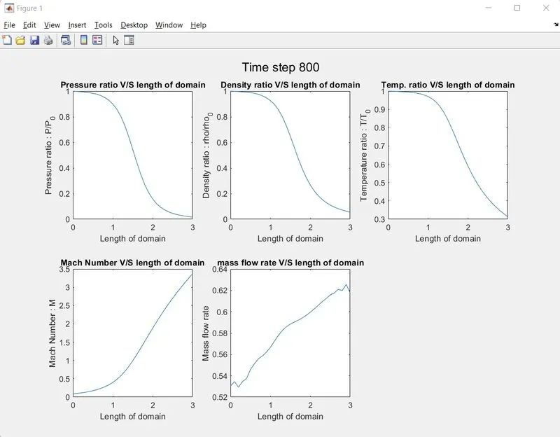
> Pressure ratio, density ratio & temperature ratio decrease along the length of the nozzle.
> Mach No. increases along the length of the nozzle & Mach No ~ 1 at the throat section.
> Mass flow rate increases along the length of the domain (but by a small factor i.e negligible as compared to non-conservative flow field)
3) Mass flow rate comparison
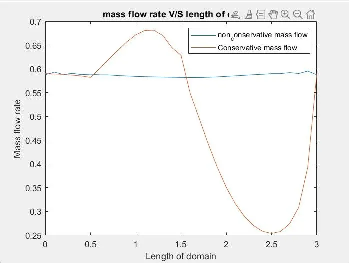
> Comparing the mass flow rate of conservative & non- conservative flow fields. We can say that it remains fairly constant for non-conservative case & varying in the case of the conservative flow field.
4) Simulation time comparison
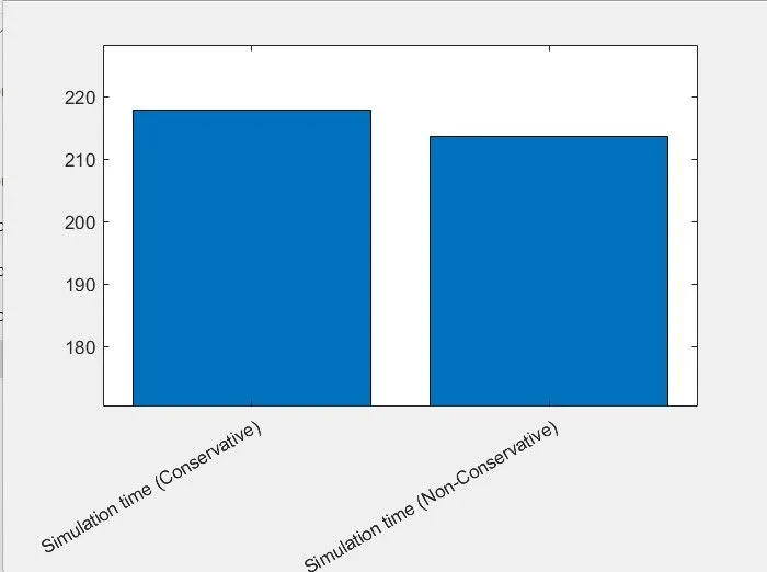
> Simulation time for conservative flow field is greater than non-conservative flow field.