Challenge

Week 7 - Simulation of a 1D Super-sonic nozzle flow simulation using Macormack Method

MMayank Singh6 Apr 2022

We are to simulate a 1D Supersonic nozzle flow using Macormack Method. Let us first understand the MacCormack Method.

MACCORMACK METHOD:

MacCormack method is a discretizing scheme used in Computational Fluid Dynamics to sole hyperbolic partial differential equations numerically. Consider a First order hyperbolic partial differential equation:

`(delu)/(delt) +a((delu)/(delx)) = 0`

The MacCormack method requires the use of two steps namely the Predictor Step and Corrector Step.

Predictor Step: The predictor step gives a provisional value at timestep `n+1`

`u_i^(n+1) = u_i^n - a/(Deltax)(u_(i+1)^n - u_i^n)`

and then update the solution:

`overline u = u_0 + u_i^(n+1) *Deltat`

where, `u_0` is the initial condition.

Corrector Step: Corrector step corrects the predicted value in the predictor step according to the equation, and uses backward difference

`overline u_i^(n+1) = overline u_i^n - a/(Deltax)(overline u_i^n - overline u_(i-1)^n)`

The actual solution is derived by calculating the average of the corrector and predictor step.

`u_(av) = (u_i^(n+1) + overline u_i^(n+1))/2`

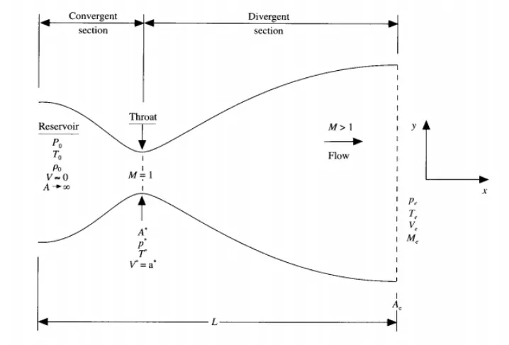
NOZZLE SCHEMATIC:

INITIAL AND BOUNDARY CONDITIONS:

The initial and boundary condition given to us for both non-conservative and conservative cases are recorded and coded into the main-script of our program as follows:

Main Script:

clear all
close all
clc

% Pre-Requisites:
n = 31;  % Node Points
x = linspace(0,3,n); % Mesh
dx = x(2) - x(1); % Mesh SIze
gamma = 1.4;
nt = 1000; % Number of Timesteps

% nozzle shape 

a = 1 + 2.2*(x - 1.5).^2; % Nozzle Area
throat = find(a==1); %throat

% Non Conservative initial condition

rho_c = 1 - 0.3146.*x; % Desity
T_c = 1 -0.2314.*x; % Temperature
v_c = (0.1 + 1.09.*x).*T_c.^0.5; % Velocity
dt_c = min((dx.*0.5)./(sqrt(T_c)+v_c)); % Time-step for C=0.5

% non-conservative solver

mdot_nc = non_conservative_solver(x,gamma,dx,nt,a,rho_c,T_c,v_c,throat,dt_c,n);

% Conservative Initial Conditions

% Density and Temperature profile along Nozzle Length
for i=1:length(x)

    if (x(i)>=0)&&(x(i)<0.5)
        rho_n(i) = 1;
        T_n(i) = 1;

    elseif (x(i)>=0.5)&&(x(i)<=1.5)
        rho_n(i) = 1 -0.366.*(x(i)-0.5);
        T_n(i) = 1-0.167.*(x(i) - 0.5);

    elseif (x(i)>1.5)&&(x(i)<=3)
        rho_n(i) = 0.634 - 0.3879.*(x(i)-1.5);
        T_n(i) = 0.833 - 0.3507.*(x(i)-1.5);
    end
end

for i = 1:n
    v_n(i) = 0.59/(rho_n(i)*a(i)); % Velocity
    u1(i) = rho_n(i)*a(i);
    u2(i) = rho_n(i)*a(i)*v_n(i);
    u3(i) = rho_n(i)*a(i)*((T_n(i)/(gamma-1))+(0.5*gamma*v_n(i)^2));
    dT_n(i) = 0.5*(dx/((T_n(i))^(0.5)+v_n(i))); % Time-step for C=0.5
end
dt_n = min(dT_n); 

% conservative solver
mdot_c = conservative_solver(x,dx,gamma,u1,u2,u3,dt_n,rho_n,T_n,nt,throat,a,n);

figure(7)
subplot(2,1,1);
plot(x,mdot_nc,'--*','DisplayName','Non-Conservative')
title('Comparison of Mass Flow Rate')
xlabel('Nozzle Length')
ylabel('$\dot {m}$', 'Interpreter','latex')
grid on;
grid minor;
legend show;

subplot(2,1,2);
plot(x,mdot_c,'--x','DisplayName','Conservative')
xlabel('Nozzle Length')
ylabel('$\dot {m}$', 'Interpreter','latex')
grid on;
grid minor;
legend show;

NON-CONSERVATIVE SOLUTION:

The governing equations for our quasi 1D flow can be given as:

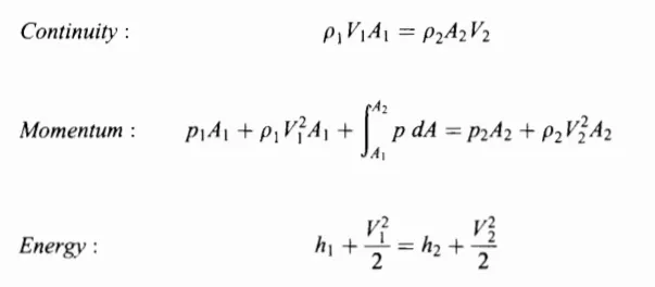
Since the flow is isentropic, we will use the isentropic gas relations:

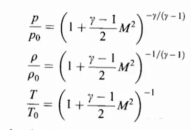
Where `M` = Mach Number

Carefully manipulating these equations mathematically, We simplify the governing equations into a single-dimensional(x term only) form and Manipulate the terms in accordance with our Isentropic Relations and finally get:

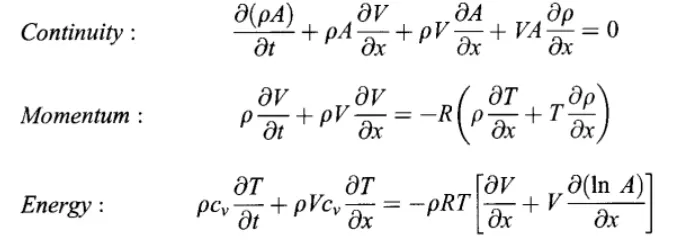
These are our Quasi 1D Isentropic flow governing equations. Further Simplifying them into their dimensionless form we get:

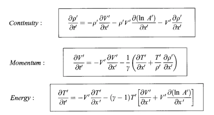
This is the non-conservative form of the governing equation, we will discretize them and compute the state throughout the domain using MacCormack Method.

We will apply this method to the non-conservative governing equations and write a MATLAB function to Solve them.

Non-Conservative Solver:

function mdot = non_conservative_solver(x,gamma,dx,nt,a,rho,T,v,throat,dt,n)

% time-loop

for i = 1:nt

    rho_init = rho;
    T_init = T;
    v_init = v;

    % Predictor Step

    for j = 2:n-1

        dvdx = (v(j+1) - v(j))/dx;
        drhodx = (rho(j+1) - rho(j))/dx;
        dTdx = (T(j+1) - T(j))/dx;
        dlogadx = (log(a(j+1)) - log(a(j)))/dx;

        %continuity equation
        p_drhodt(j) = - rho(j)*dvdx - rho(j)*v(j)*dlogadx - v(j)*drhodx;

        %Momentum Equation
        p_dvdt(j) = -v(j)*dvdx - (1/gamma)*(dTdx + (T(j)*drhodx/rho(j)));

        %energy equation
        p_dTdt(j) = -v(j)*dTdx - (gamma-1)*T(j)*(dvdx*v(j)*dlogadx);

        %update
        rho(j) = rho(j) + p_drhodt(j)*dt;
        v(j) = v(j) + p_dvdt(j)*dt;
        T(j) = T(j) + p_dTdt(j)*dt;

    end

    % Corrector Step

    for j = 2:n-1

        dvdx = (v(j) - v(j-1))/dx;
        drhodx = (rho(j) - rho(j-1))/dx;
        dTdx = (T(j) - T(j-1))/dx;
        dlogadx = (log(a(j)) - log(a(j-1)))/dx;

        %continuity equation
        c_drhodt(j) = - rho(j)*dvdx - rho(j)*v(j)*dlogadx - v(j)*drhodx;

        %Momentum Equation
        c_dvdt(j) = -v(j)*dvdx - (1/gamma)*(dTdx + (T(j)*drhodx/rho(j)));

        %energy equation
        c_dTdt(j) = -v(j)*dTdx - (gamma-1)*T(j)*(dvdx*v(j)*dlogadx);

    end

    % Average

    drhodt = (p_drhodt + c_drhodt).*0.5;
    dvdt = (p_dvdt + c_dvdt).*0.5;
    dTdt = (p_dTdt + c_dTdt).*0.5;

    % final solution

    for k = 2:n-1

        rho(k) = rho_init(k) + drhodt(k)*dt;
        v(k) = v_init(k) + dvdt(k)*dt;
        T(k) = T_init(k) + dTdt(k)*dt;

    end

    % Boundary Conditions
    %inlet

    rho(1) = 1;
    v(1) = 2*v(2) - v(3);
    T(1) = 1;

    %outlet

    rho(n) = 2*rho(n-1) - rho(n-2);
    v(n) = 2*v(n-1) - v(n-2);
    T(n) = 2*T(n-1) - T(n-2);

    % other parameters

    mdot = rho.*a.*v; % Mass Flow Rate
    p = rho.*T; % Pressure
    M = v./(sqrt(T)); % Mach Number

    % At throat

    rho_t(i) = rho(throat);
    T_t(i) = T(throat);
    v_t(i) = v(throat);
    mdot_t(i) = mdot(throat);
    p_t(i) = p(throat);
    M_t(i) = M(throat);


    % PLOTS
    
    figure(1)
    if i==100
        plot(x,mdot,'--x','DisplayName',"100t")
        hold on
    elseif i==200
        plot(x,mdot,'--x','DisplayName',"200t")
        hold on
    elseif i==300
        plot(x,mdot,'--x','DisplayName',"300t")
        hold on
    elseif i==400
        plot(x,mdot,'--x','DisplayName',"400t")
        hold on
    elseif i==500
        plot(x,mdot,'--x','DisplayName',"500t")
        hold on
    elseif i==600
        plot(x,mdot,'--x','DisplayName',"600t")
        hold on
    elseif i==700
        plot(x,mdot,'--x','DisplayName',"700t")
        hold on
    elseif i==800
        plot(x,mdot,'--x','DisplayName',"800t")
        hold on
    elseif i==900
        plot(x,mdot,'--x','DisplayName',"900t")
        hold on
    elseif i==1000
        plot(x,mdot,'--x','DisplayName',"1000t")
        hold on
    end

    title('Time-Wise Variation of Mass Flow Rate along Nozzle Length (Non-Conservative)')
    xlabel('Nozzle Length')
    ylabel('$\dot {m}$', 'Interpreter','latex')
    grid on;
    grid minor;
    legend show;
end

figure(2)

% Density
plot(linspace(1,nt,nt),rho_t,'DisplayName',"Density")
hold on;

% Pressure
plot(linspace(1,nt,nt),p_t,'DisplayName',"Pressure")
hold on;

% Temperature
plot(linspace(1,nt,nt),T_t,'DisplayName',"Temperature")
hold on;

% Mach Number
plot(linspace(1,nt,nt),M_t,'DisplayName',"Mach Number")
hold on;

title('Flow Parameters at Throat vs Time  (Non-Conservative)')
xlabel('Time')
ylabel('Magnitude')
grid on;
grid minor;
legend show;

figure(3)

% Density
plot(x,rho,'DisplayName',"Density")
hold on;

% Pressure
plot(x,p,'DisplayName',"Pressure")
hold on;

% Temperature
plot(x,T,'DisplayName',"Temperature")
hold on;

% Mach Number
plot(x,M,'DisplayName',"Mach Number")
hold on;

title('Flow Parameters vs Distance (Non-Conservative)')
xlabel('Nozzle length')
ylabel('Magnitude')
grid on;
grid minor;
legend show;

CONSERVATIVE SOLUTION:

For Conservative Solution we will simplify our governing equations and use substitute variables for complex terms as shown below:

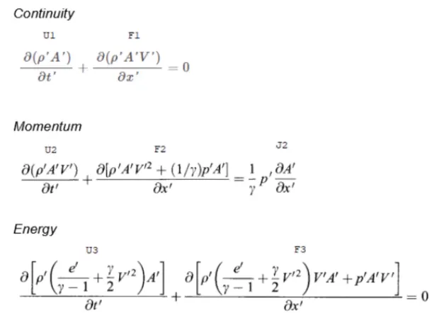
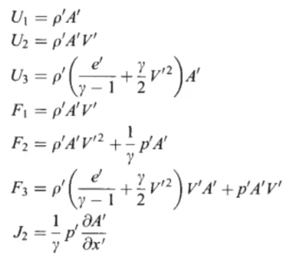
We have introduced 6 substitute variables which can be written as:

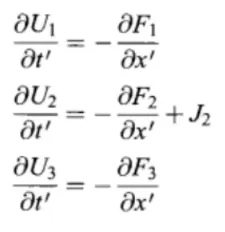
Now we will rewrite our governing equations using the above relations:

Lastly, for ease of numerical analysis we will express F1, F2, F3 and J2 in terms of U1, U2, and U3:

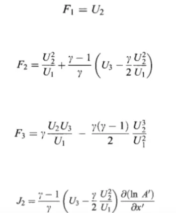
We will incorporate these equations in our conservative solver.

Conservative Solver:

function [mdot] = conservative_solver(x,dx,gamma,u1,u2,u3,dt,rho,T,nt,throat,a,n)

for i=1:nt

    u1_init = u1;
    u2_init = u2;
    u3_init = u3;

    f1 = u2;
    f2 = ((u2.^2)./(u1)) + (((gamma-1)/gamma).*(u3-((gamma/2).*(((u2.^2)./u1)))));
    f3 = ((gamma.*u2.*u3)./u1) - (gamma.*(gamma-1)/2)*((u2.^3)./u1.^2);

    % Predictor Step

    for j=2:n-1

        df1dx = (f1(j+1) - f1(j))/dx;
        df2dx = (f2(j+1) - f2(j))/dx;
        df3dx = (f3(j+1) - f3(j))/dx;

        p_du1dt(j) = -df1dx;
        j2(j) = ((1/gamma)*rho(j)*T(j)*((a(j+1)-a(j))/dx));
        p_du2dt(j) = -df2dx + j2(j);
        p_du3dt(j) = -df3dx;

        u1(j) = u1(j) + p_du1dt(j)*dt;
        u2(j) = u2(j) + p_du2dt(j)*dt;
        u3(j) = u3(j) + p_du3dt(j)*dt;

    end

    % update

    rho = u1./a;
    v = u2./u1;
    T = (gamma-1).*((u3./u1)-(0.5*gamma.*v.^2));

    f1 = u2;
    f2 = ((u2.^2)./(u1)) + (((gamma-1)/gamma).*(u3-((gamma/2).*(((u2.^2)./u1)))));
    f3 = ((gamma.*u2.*u3)./u1) - (gamma.*(gamma-1)/2)*((u2.^3)./u1.^2);
    
    % Corrector Step
    for j=2:n-1

        df1dx = (f1(j) - f1(j-1))/dx;
        df2dx = (f2(j) - f2(j-1))/dx;
        df3dx = (f3(j) - f3(j-1))/dx;

        c_du1dt(j) = -df1dx;
        j2(j) = ((1/gamma)*rho(j)*T(j)*((a(j)-a(j-1))/dx));
        c_du2dt(j) = -df2dx + j2(j);
        c_du3dt(j) = -df3dx;

    end

    % Average

    du1dt = (p_du1dt + c_du1dt)*0.5;
    du2dt = (p_du2dt + c_du2dt)*0.5;
    du3dt = (p_du3dt + c_du3dt)*0.5;

    % Final Solution

    for k = 2:n-1

        u1(k) = u1_init(k) + du1dt(k)*dt;
        u2(k) = u2_init(k) + du2dt(k)*dt;
        u3(k) = u3_init(k) + du3dt(k)*dt;

    end

    % Boundary Conditions
    %inlet

    u1(1) = rho(1)*a(1);
    u2(1) = 2*u2(2) - u2(3);
    v(1) = u2(1)/(rho(1)*a(1));
    u3(1) = u1(1)*((T(1)/(gamma-1))+((gamma*0.5)*v(1)^2));

    %outlet

    u1(n) = 2*u1(n-1) - u1(n-2);
    u2(n) = 2*u2(n-1) - u2(n-2);
    u3(n) = 2*u3(n-1) - u3(n-2);

    % update

    rho = u1./a;
    v = u2./u1;
    T = (gamma-1).*((u3./u1)-(0.5*gamma.*v.^2));

    % Other Parameters

    mdot = rho.*v.*a; % Mass Flow Rate
    p = rho.*T; % Pressure
    M = v./(sqrt(T)); % Mach Number

    % AT throat

    rho_t(i) = rho(throat);
    T_t(i) = T(throat);
    v_t(i) = v(throat);
    mdot_t(i) = mdot(throat);
    p_t(i) = p(throat);
    M_t(i) = M(throat);
    
    figure(4)
    if i==100
        plot(x,mdot,'--x','DisplayName',"100t")
        hold on
    elseif i==200
        plot(x,mdot,'--x','DisplayName',"200t")
        hold on
    elseif i==300
        plot(x,mdot,'--x','DisplayName',"300t")
        hold on
    elseif i==400
        plot(x,mdot,'--x','DisplayName',"400t")
        hold on
    elseif i==500
        plot(x,mdot,'--x','DisplayName',"500t")
        hold on
    elseif i==600
        plot(x,mdot,'--x','DisplayName',"600t")
        hold on
    elseif i==700
        plot(x,mdot,'--x','DisplayName',"700t")
        hold on
    elseif i==800
        plot(x,mdot,'--x','DisplayName',"800t")
        hold on
    elseif i==900
        plot(x,mdot,'--x','DisplayName',"900t")
        hold on
    elseif i==1000
        plot(x,mdot,'--x','DisplayName',"1000t")
        hold on
    end

    title('Time-Wise Variation of Mass Flow Rate along Nozzle Length (Conservative)')
    xlabel('Nozzle Length')
    ylabel('$\dot {m}$', 'Interpreter','latex')
    grid on; 
    grid minor;
    legend show;
end

figure(5)

% Density
plot(linspace(1,nt,nt),rho_t,'DisplayName',"Density")
hold on;

% Pressure
plot(linspace(1,nt,nt),p_t,'DisplayName',"Pressure")
hold on;

% Temperature
plot(linspace(1,nt,nt),T_t,'DisplayName',"Temperature")
hold on;

% Mach Number
plot(linspace(1,nt,nt),M_t,'DisplayName',"Mach Number")
hold on;

title('Flow Parameters at Throat vs Time (Conservative)')
xlabel('Time')
ylabel('Magnitude')
grid on;
grid minor;
legend show;

figure(6)

% Density
plot(x,rho,'DisplayName',"Density")
hold on;

% Pressure
plot(x,p,'DisplayName',"Pressure")
hold on;

% Temperature
plot(x,T,'DisplayName',"Temperature")
hold on;

% Mach Number
plot(x,M,'DisplayName',"Mach Number")
hold on;

title('Flow Parameters vs Distance (Conservative)')
xlabel('Nozzle Length')
ylabel('Magnitude')
grid on;
grid minor;
legend show;

RESULTS:

Non-Conservative Solution:

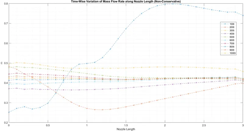
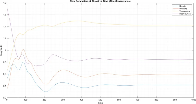
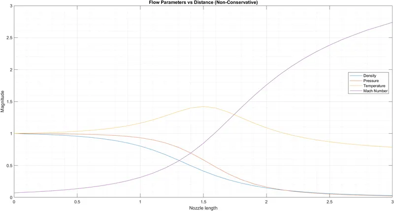
From the above plots it can be inferred that:

The Steady-State is acheived post 500th timestep.
The density, pressure and Temperature of the flow decreases as it moves along the nozzle length and the mach number shoots up.

Conservative Solution:

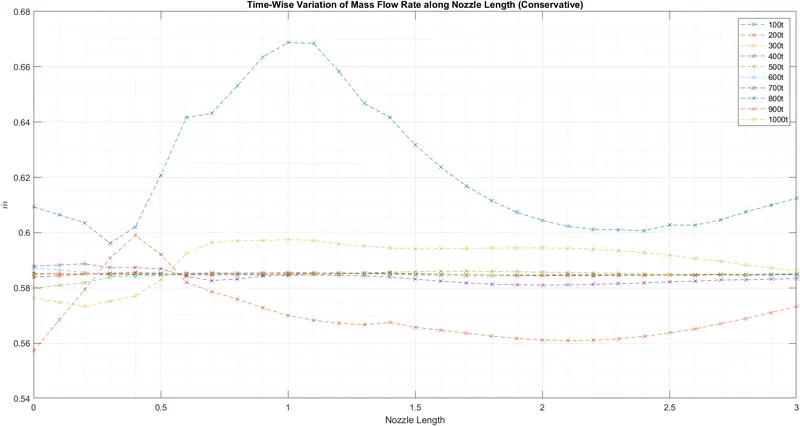
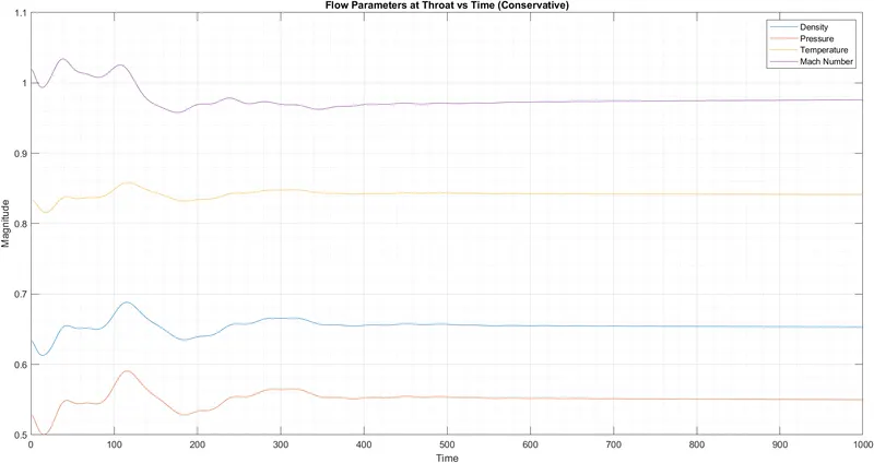
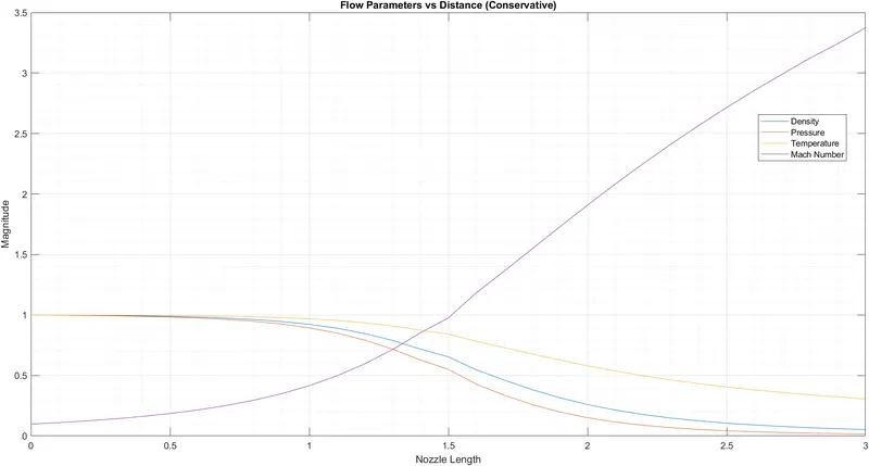
Since the problem statement is same we don't see much difference in our findings for conservative flow compared to non-conservative flow. Fluctuation in magnitude is oobservable but the trend remains same.

Comparison of Mass Flow Rates in both modes:

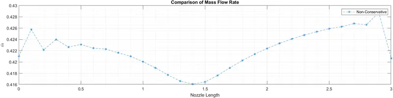
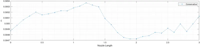
On comparing the Mass Flow rate, we see some variation in the trend as well as magnitude between the two solvers. This can be attributed to the change in initial and boundary conditions for Conservative Solver.

Grid Independence Test:

To check dependency on grid, we will compare the mass flow rate obtained through the solution for a varying number of gridpoints.

n	`dot m_c`	`dot m_(nc)`
31	0.5850	0.4221
51	0.5831	0.4049
61	0.5832	0.4354
101	0.5865	0.4730

From these tabulated results we can see that conservative solution shows comparatively more grid indepence than non-conservative solution. This concludes our study.

Week 7 - Simulation of a 1D Super-sonic nozzle flow simulation using Macormack Method

Ship work like this
in your own course.

Talk to a career counsellor

Ship work like thisin your own course.

Talk to a career counsellor

Ship work like this
in your own course.