Week 1- Mixing Tee

AIM:

For this challenge, we have created two versions of the mixing tee. One of them is longer than the other.

We will set up steady-state simulations to compare the mixing effectiveness when the hot inlet temperature is 36⁰C & the Cold inlet is 19⁰C.

We Use the k-epsilon and k-omega SST model for the first case and, based on the results, use the more suitable model for the other case.

1. Case 1
   • Short mixing tee with a hot inlet velocity of 3m/s.
   • Momentum ratio of 2, 4.
2. Case 2
   • Long mixing tee with a hot inlet velocity of 3m/s.
   • Momentum ratio of 2, 4.

Momentum ratio = velocity at cold inlet / velocity at hot inlet

Lastly, we compare the following values from the 2 cases.

1. Cell count
2. Average outlet temperature
3. Number of iterations for convergence

INTRODUCTION:

Mixing Tees are used to mix two fluids at different temperatures effectively and are used extensively in the HVAC industry. We will be calculating the effectiveness of this geometry and determining the best parameters for the highest efficiency. We have two models with different lengths to choose the effect of length. Two turbulent models to determine the most accurate result and varying momentum ratios to determine the ideal velocity for maximum effectiveness.

THEORY:

Turbulence Models: Turbulence models are mathematical models used to predict the nature of turbulence. They are extensively used to simulate real-life turbulent flows in CFD applications.

For our problem, we are comparing two turbulence models, viz. K-epsilon (k-ε) turbulence model and k–omega (k–ω) turbulence model

K-epsilon (k-ε) TURBULENCE MODEL:

k-ε model is the most common turbulence model used in CFD applications. It was initially designed to improve the mixing-length model and also to find a substitute for prescribing turbulence length algebraically in moderate to high-complexity flows. It is a two-equation model where the first transported variable is kinetic energy(k), and the second variable is the rate of turbulent kinetic energy dissipation (ε).

It is also the simplest turbulence model for which only initial or boundary conditions are needed.

For turbulent kinetic energy k,

For dissipation,

where

represents velocity component in the corresponding direction

represents the component of the rate of deformation

represents eddy viscosity

For our study, we will be using the k-ε Realisable model, which provides improved predictions for the spreading rate of both planar and round jets. It also shows superior performance for flows involving rotation, boundary layers under adverse solid pressure gradients, separation, and recirculation. In virtually every measure of comparison, Realisable k-ɛ demonstrates a superior ability to capture the mean flow of the complex structures.

k–omega (k–ω) TURBULENCE MODEL:

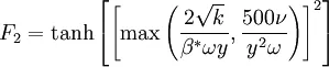
The k-omega turbulence model is similar to the k-epsilon model, as it requires two transport equations, i.e. one for kinetic energy (k) and a specific rate of dissipation (ω). It is used when wall effects are present within the case. It is one of the standard turbulence models used for Reynolds-averaged Navier-Stokes (RANS) flows. There are many variations of k–ω turbulence models; for our study, we will be focusing on the k–ω SST Model.

SST stands for Shear Stress Transport. The k−ω SST model better predicts flow separation than most RANS models and accounts for accuracy in adverse pressure gradients.

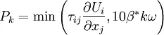
For Turbulent Kinetic Energy(k):

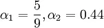
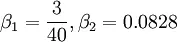
For dissipation (ω):

where,

SETTING UP THE PROJECT:

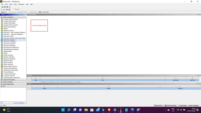
1. We will open ANSYS Workbench and select the Fluid Flow (FLUENT) module and drag it to the workspace:

This will give us the barebones skeletal framework of our workflow:

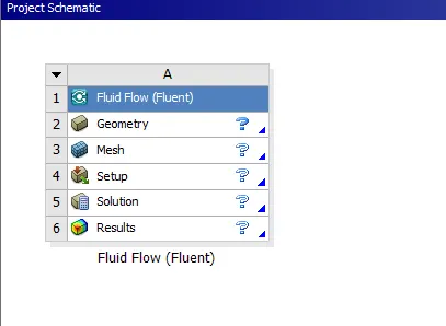
2. ANSYS automatically lists the necessary steps to be done and the order to perform them. First, we begin by setting up the geometry. Double-clicking on geometry from the list will open up the ANSYS built-in CAD tool called Spaceclaim.

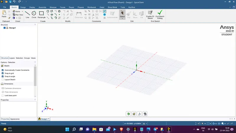
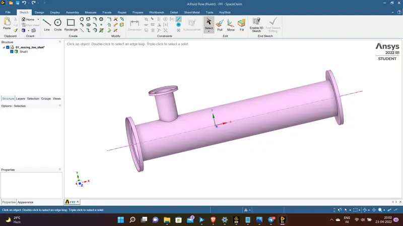
We use the file menu, and using the open command, we navigate to the location where our mixing-tee geometry file is located and open it. Spaceclaim then displays the geometry for further modifications if required:

Once we have our geometry in place, we need to extract the fluid volume from it since our simulation is only based on fluid volume. We can do this by navigating to the prepare menu and selecting volume extract:

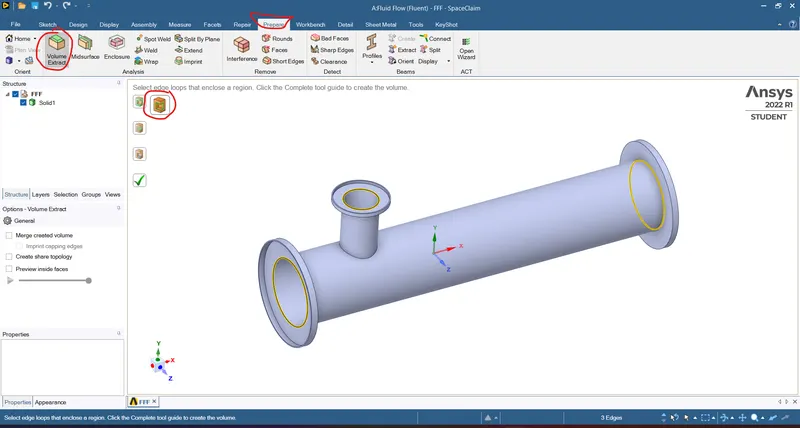
As shown above, click on the select edges on the top right and select all the edges that enclose the volume, and we can extract the volume as shown below:

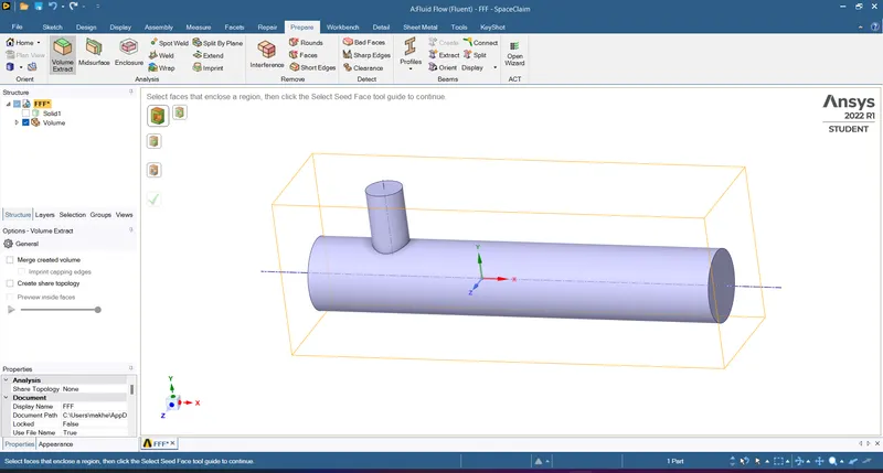
As we complete the corresponding step, ANSYS offers a green tick to show that this part is done, and we can move on to the next step:

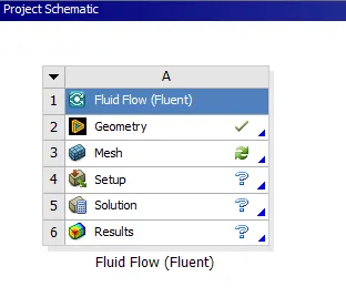
The next step is Meshing; The geometry needs to be broken down into more minor elements, and then calculations are done on each component. Eventually, the solution is derived by summing up the results. Double-clicking on mesh opens the ANSYS Meshing tool:

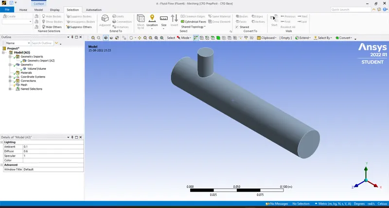
3. First, we will identify our boundaries and define them using face selection (Ctrl+f) and selecting the boundaries:

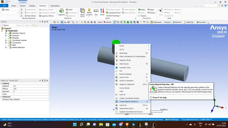
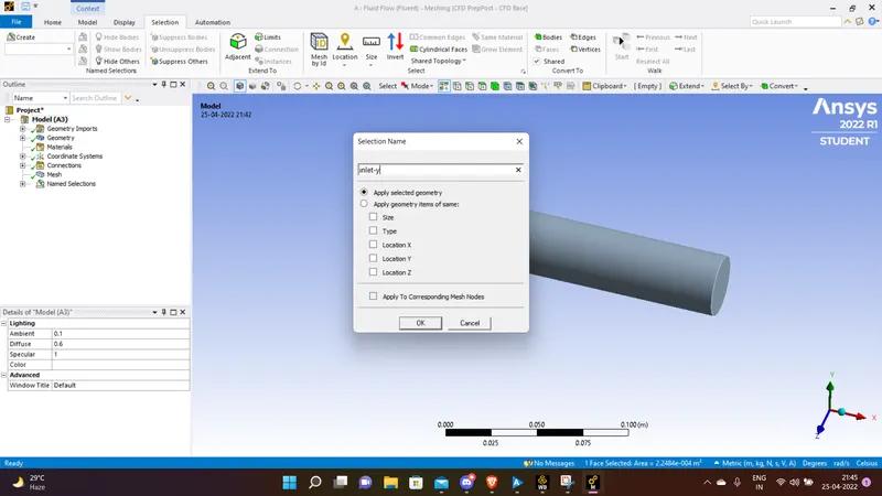
Similarly, we name our walls, the other inlet and the outlet.

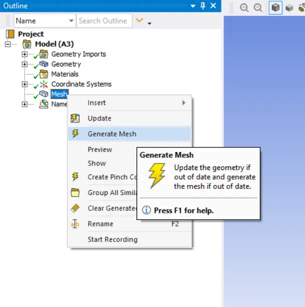
4. We can generate the mesh using the mesh menu from the project outline on the left. This will generate a mesh with the default element size:

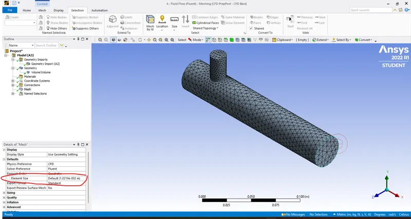
For accurate results, we need to refine our mesh. We can change the element size from the menu highlighted above. An important point to note is that the ANSYS student license allows for only 512 elements/nodes per problem, so we must keep within those limits. We will also use element metrics to determine the quality of the mesh:

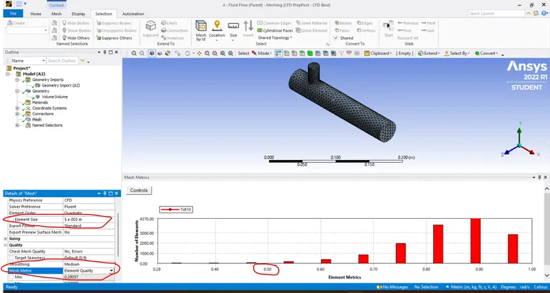
Quality higher than 0.5 will suffice; since most of our elements lie beyond 0.5, we can proceed to the next step.

SETUP AND SOLUTION:

Now we have the essential prerequisites for our case, and we will define the physics and boundary conditions for our study.

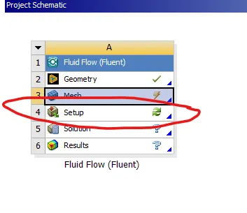
This will open up ANSYS FLuent: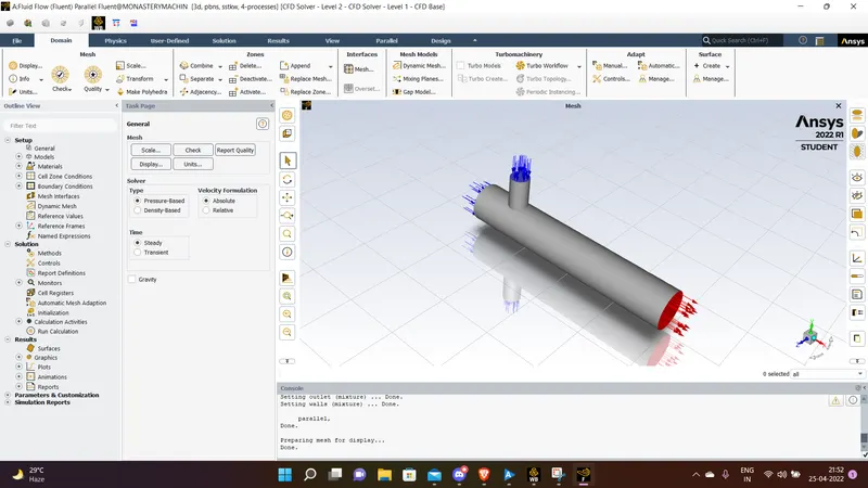

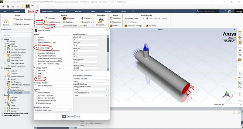
5. Next, we will be defining the physics for our flow; first, we will define the turbulence model as follows:

6. Next, we set up the boundary conditions:

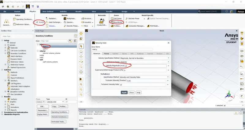
As shown above, we will check in the Energy Check-box since we are interested in Temperature Profile and set the Temperature for inflow:

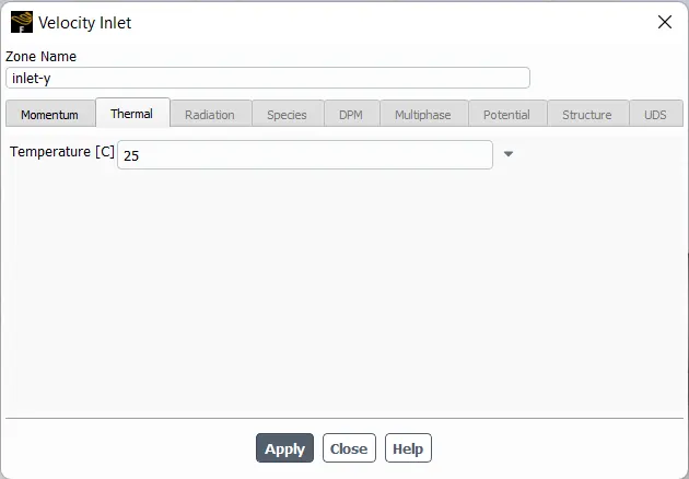
Similarly, we will set the other inlet at `10^0` C, and for the Momentum Ratio to be 2, we will assign the cold inlet velocity at 6 m/s.

7. With our case set up formally, we will create a definition that will help us check the output in a way we understand, for example, showing us the outlet temperature as the solution goes:

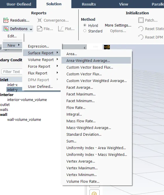
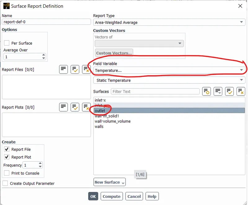
8. We will finalise it by initialising our model via the hybrid method and then perform the solution calculation using the right-most calculate button.

9. We will see our defined plot progress as the calculation proceeds:

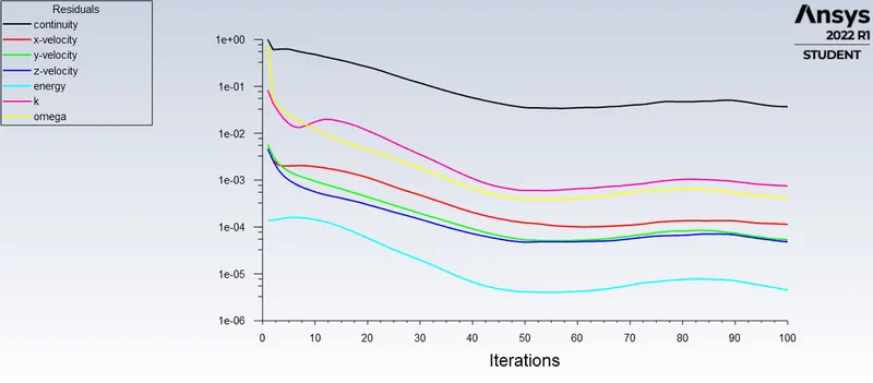
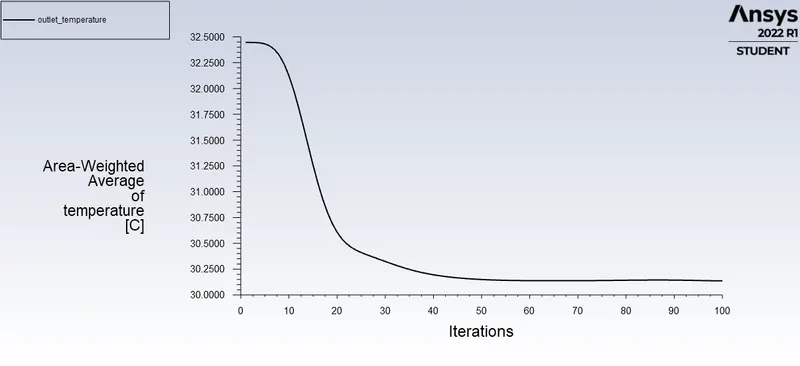
These plots show that the residuals become pretty stable beyond the 60th iteration.

POST-PROCESSING:

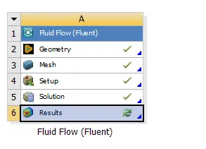
10. We will now need to post-process the result for more physical and understandable results using the results module, which will open Ansys Post:

11. We need first to draw planes and lines in the Ansys post, along which we will be plotting our charts and contours using the location menu:

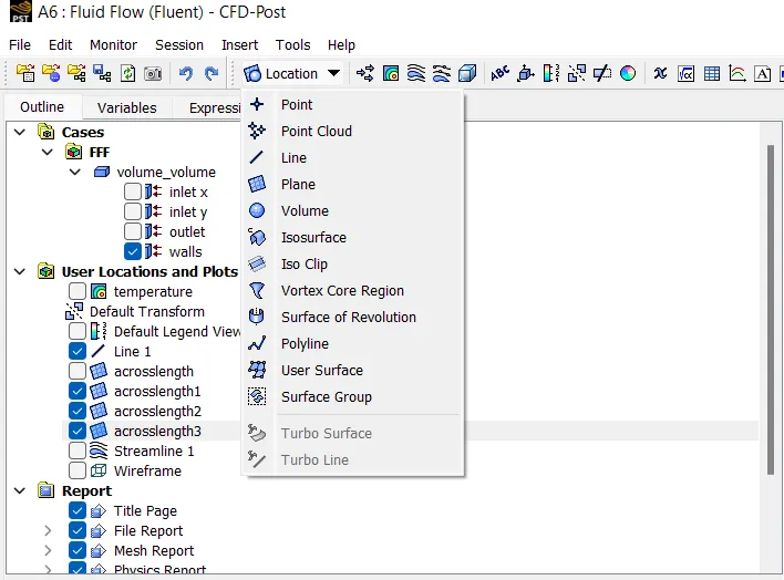
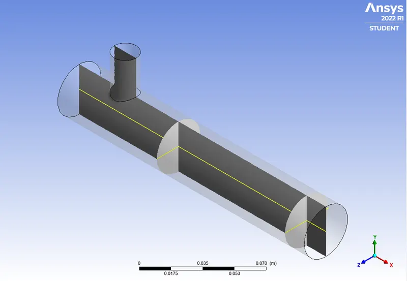
We will draw a line along the length of our geometry and an XY plane. Then, we will define 2 YZ planes at the middle and end of our geometry to plot the parameters across the pipe:

CHARTS:

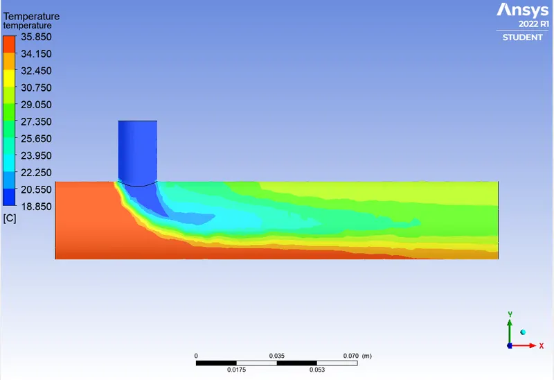
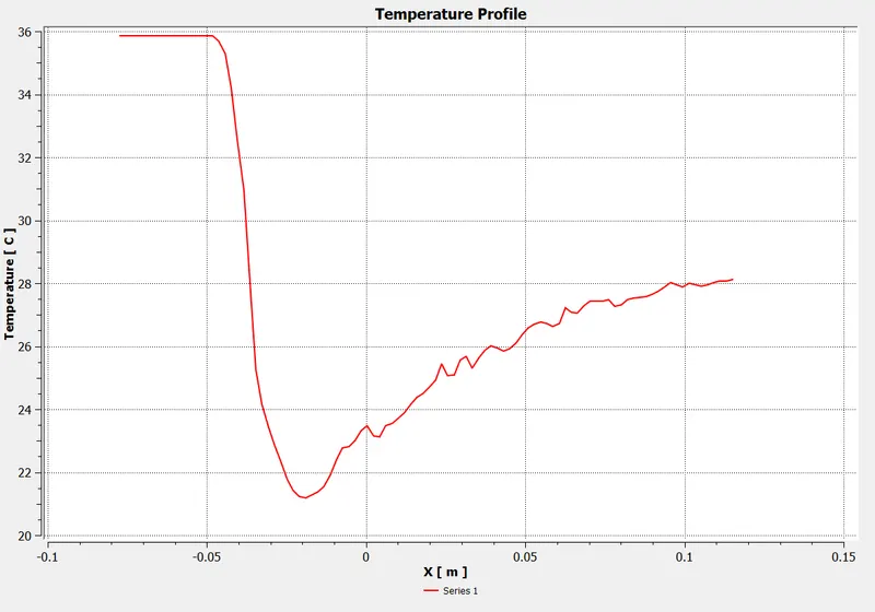
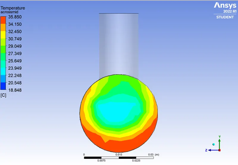
Temperature Plots:

Across Length:

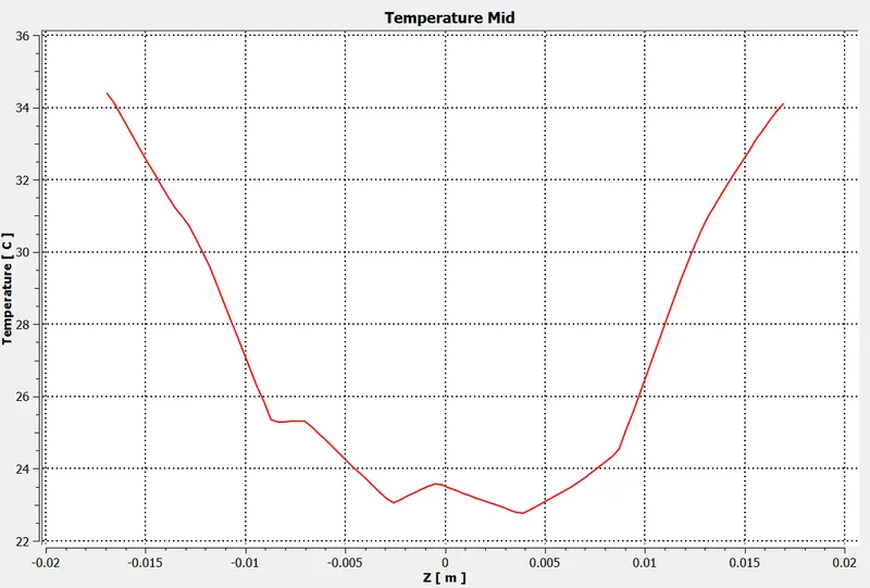
Across Mid:

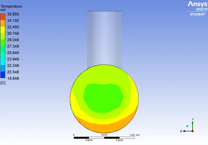
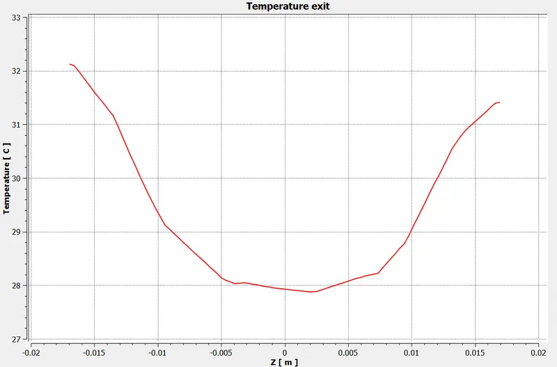
Near Exit:

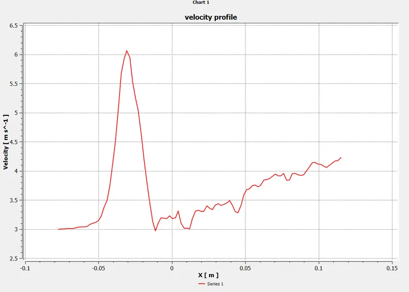
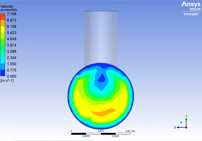
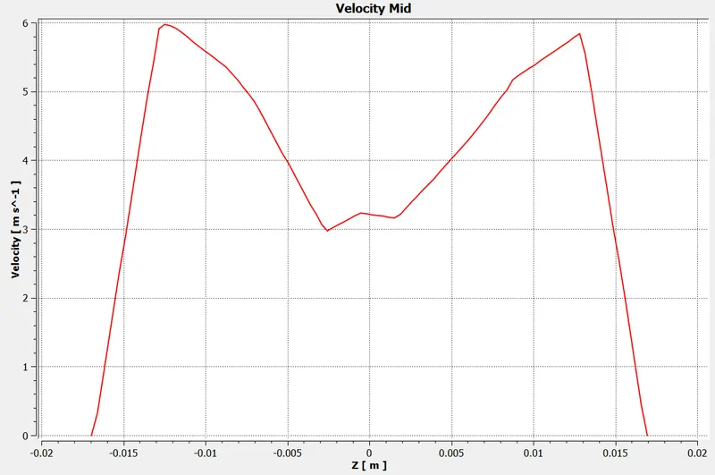
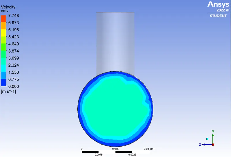
Velocity Plots:

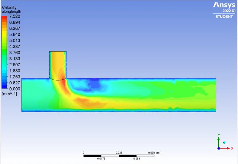
Along Length:

Across Mid:

Near Exit:

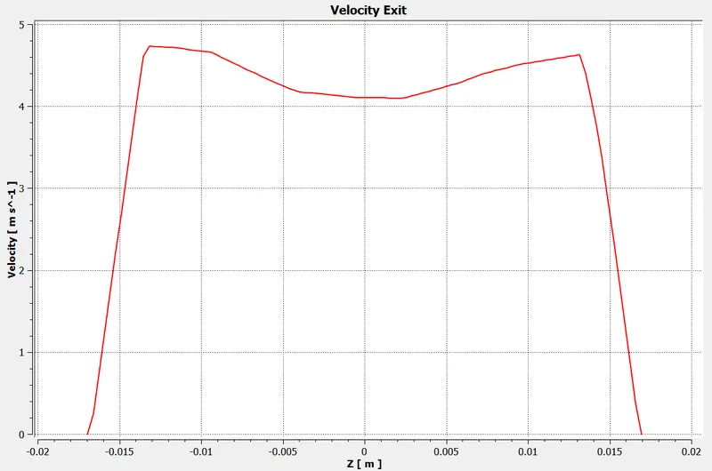
We will now calculate the solution using the K-epsilon method and compare the results.

CONVERGENCE:

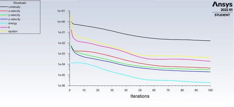
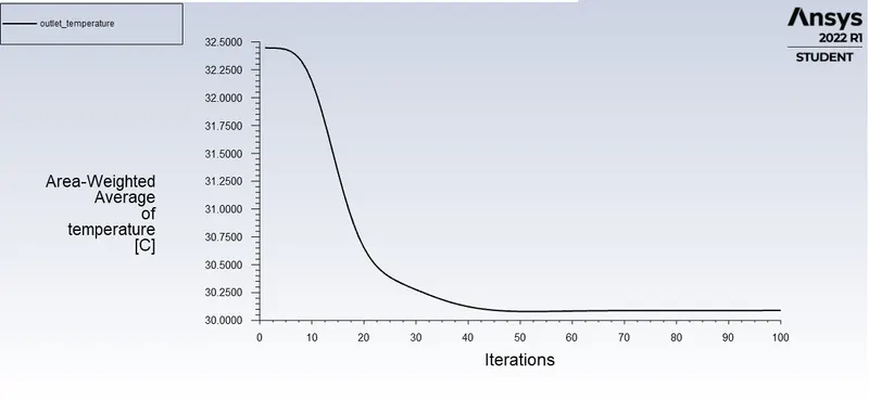
As we see, the convergence criterion is similar to that of K-omega, and we don't see any noticeable difference with the solution converging around the 60th iteration

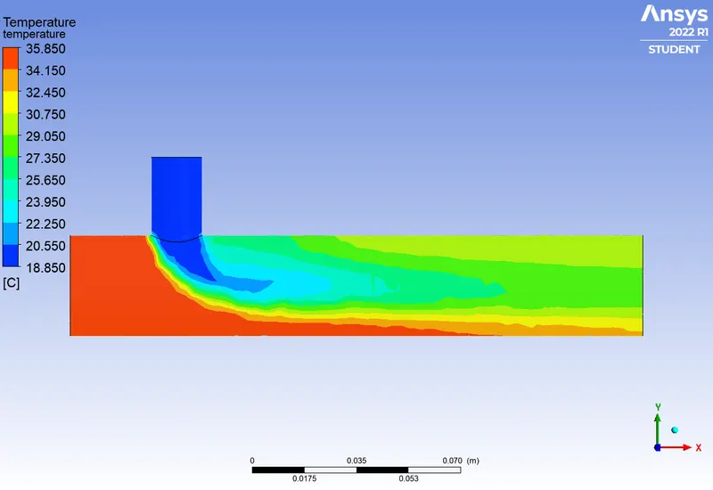
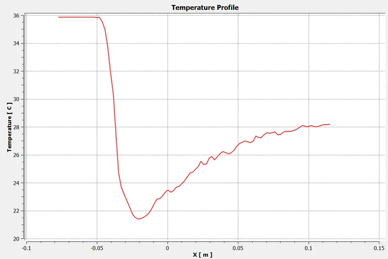
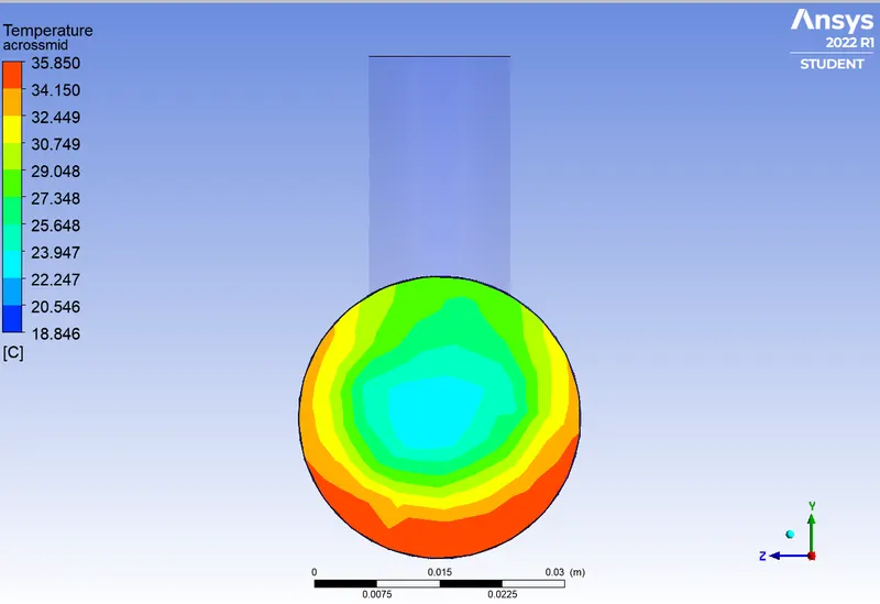
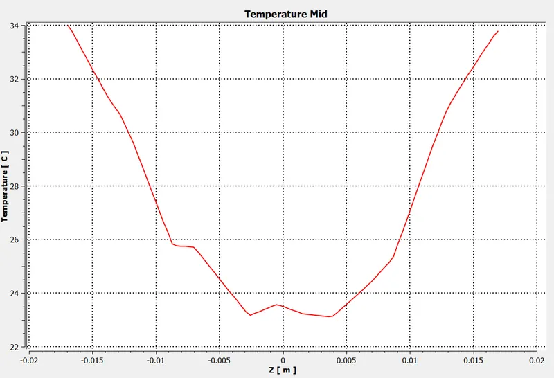
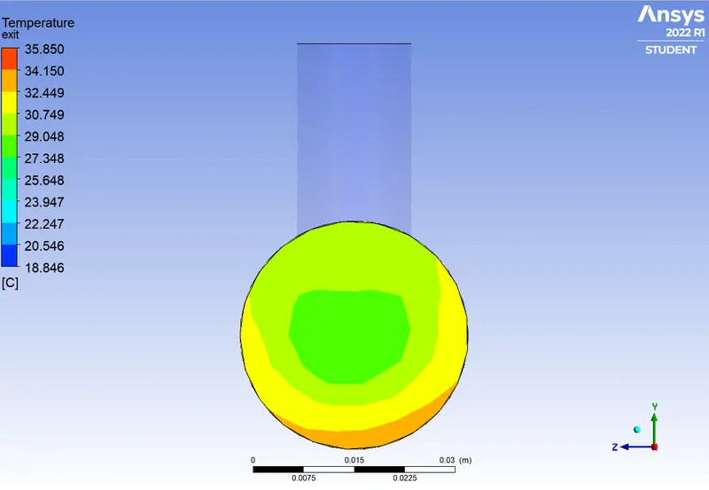
TEMPERATURE PLOTS:

Along the length:

Mid:

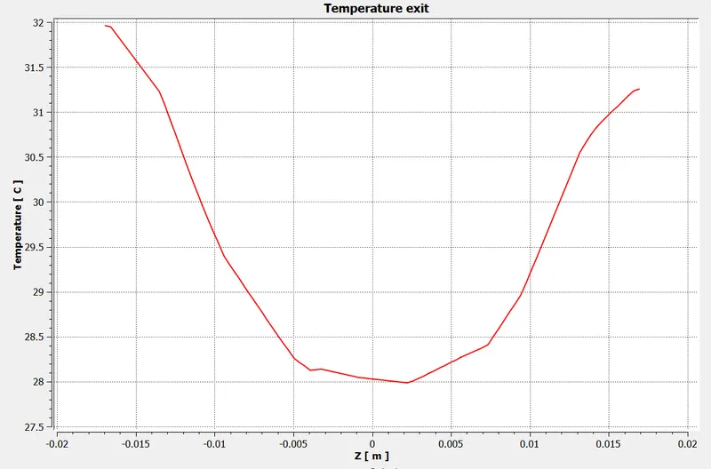
Exit:

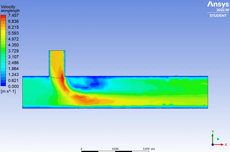
VELOCITY PLOTS:

Along Length:

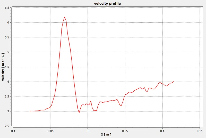
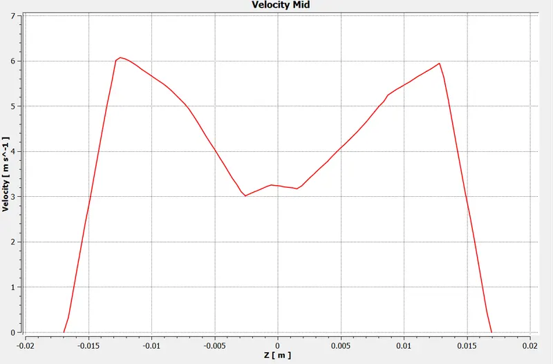
Mid:

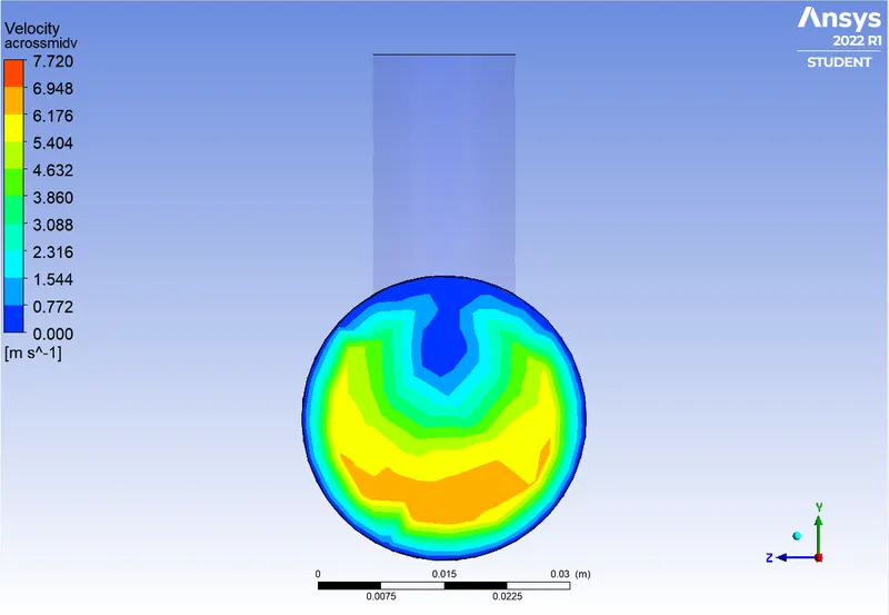
Exit:

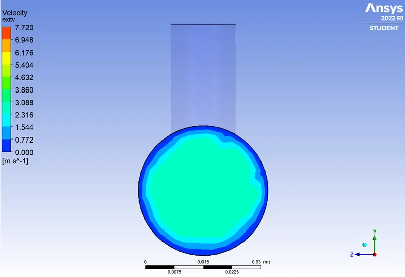
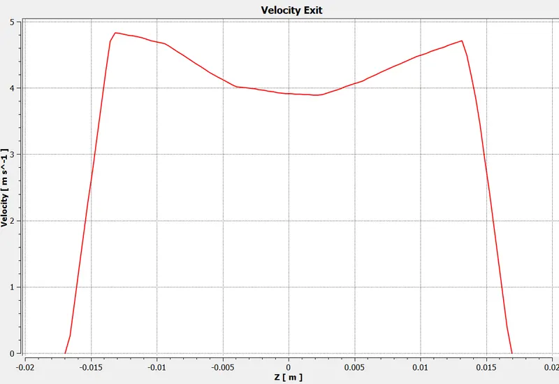
We don't find any considerable changes in the results and convergence time as we compare these results. However, the k–ω SST model is more effective when boundary separation and walls are in question than its counterpart in various studies. Therefore, We will go ahead with the k–ω SST model.

MOMENTUM RATIO = 4:

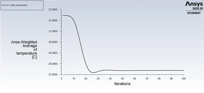
Let us move on to the second criterion; we have already established results for Momentum Ratio = 2. We will now change the cold inlet velocity to 12 m/s and see the effect it has on our simulation:

CONVERGENCE:

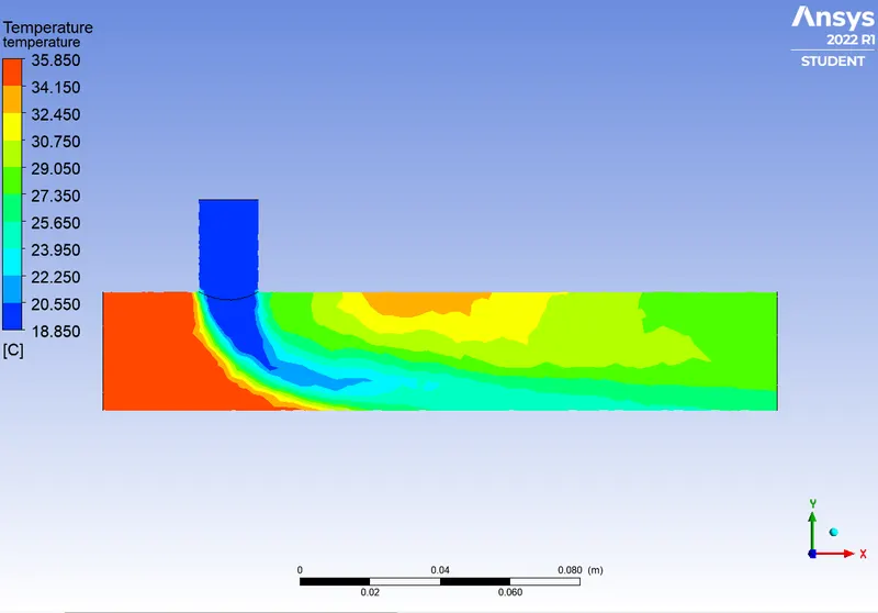
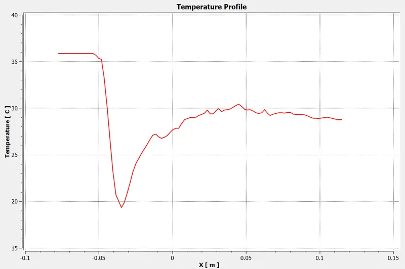
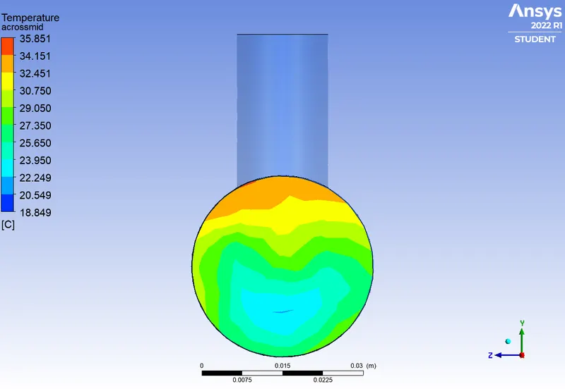
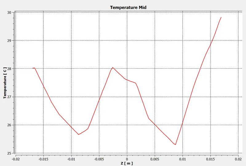
TEMPERATURE PLOTS:

Mid:

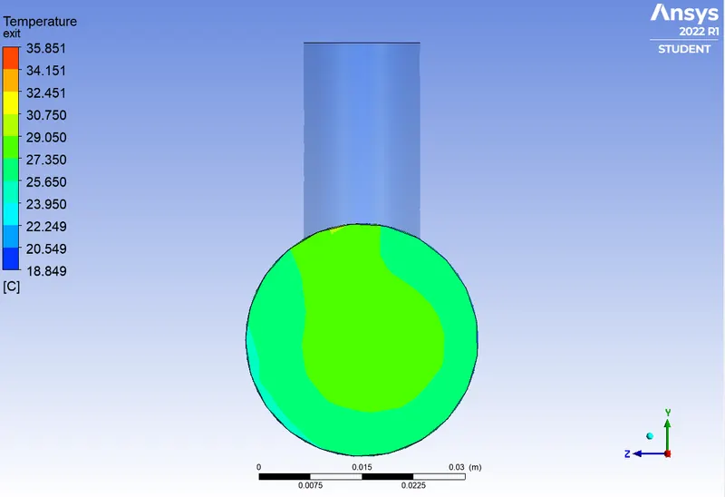
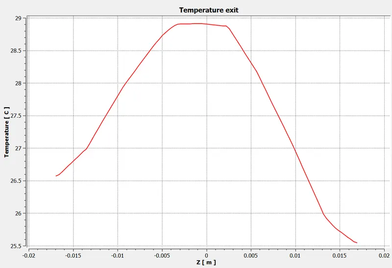
Exit:

VELOCITY PLOTS:

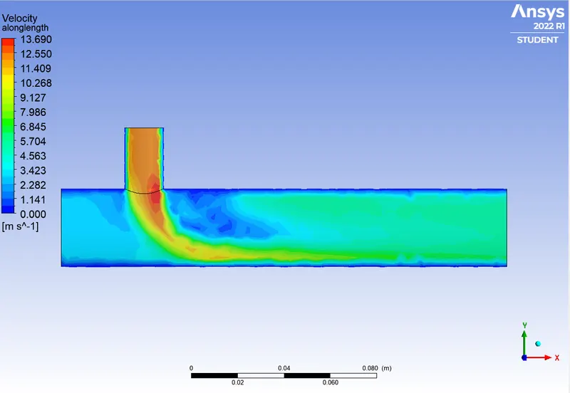
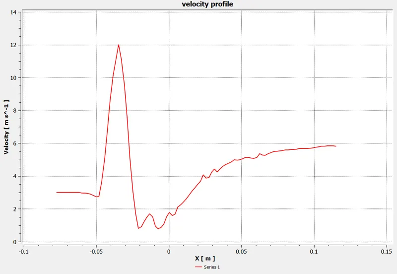
Along Length:

Mid:

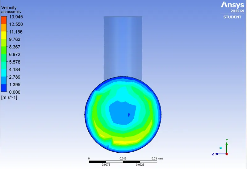
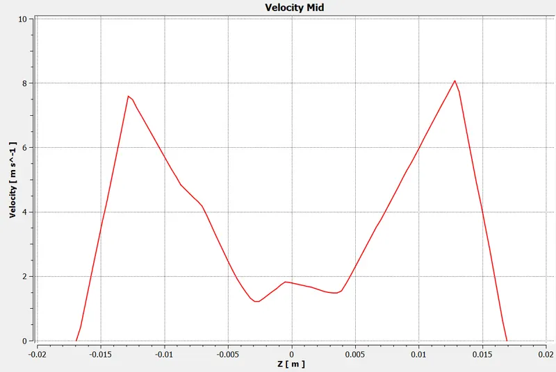
Exit:

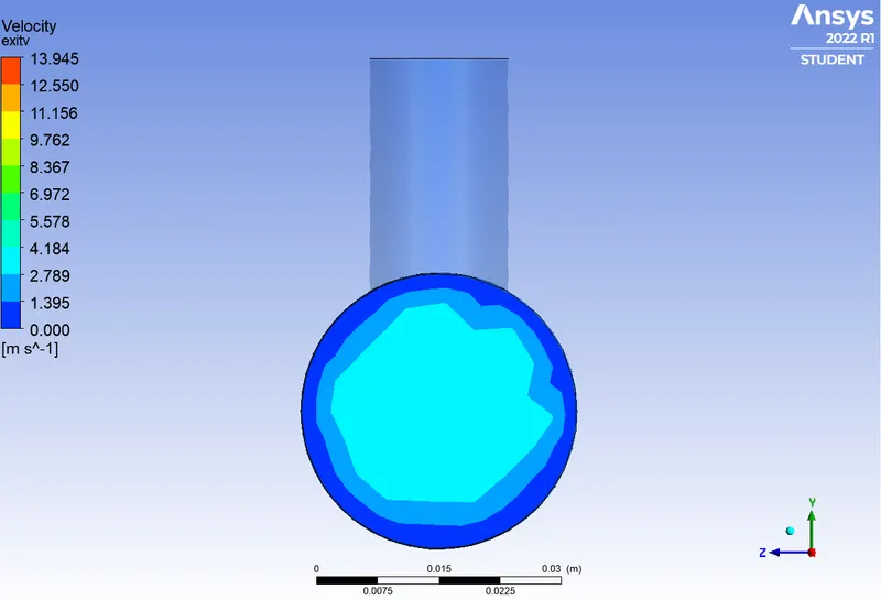
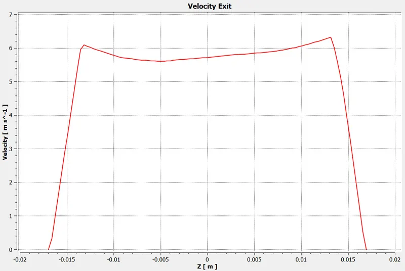
Comparing these results with the earlier ones, we can easily infer that the mixing is more efficient at a higher momentum ratio as the contours are more evened out both in the case of Velocity as Well as Temperature.

MESS INDEPENDENT STUDY:

Checking with 2 cases of element size 5 mm and 3 mm, there appears to be no significant difference in the solution. Hence, further refinement of mesh is unnecessary.

CASE II - Longer Tee:

Next, for case 2, we will test the effect of the Tee length and use a slightly longer geometry to simulate the flow:

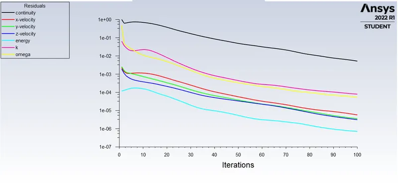
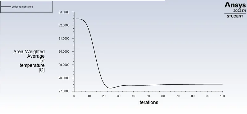
CONVERGENCE:

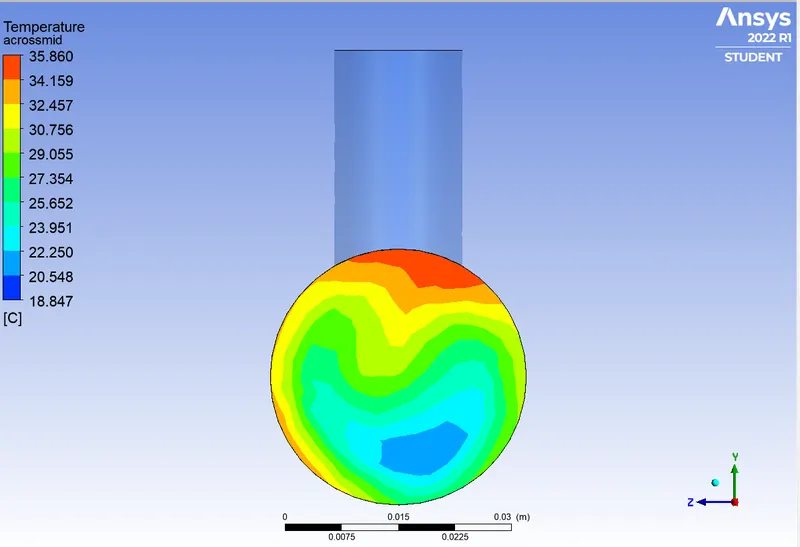
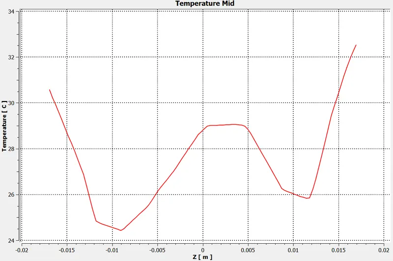
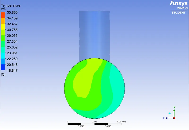
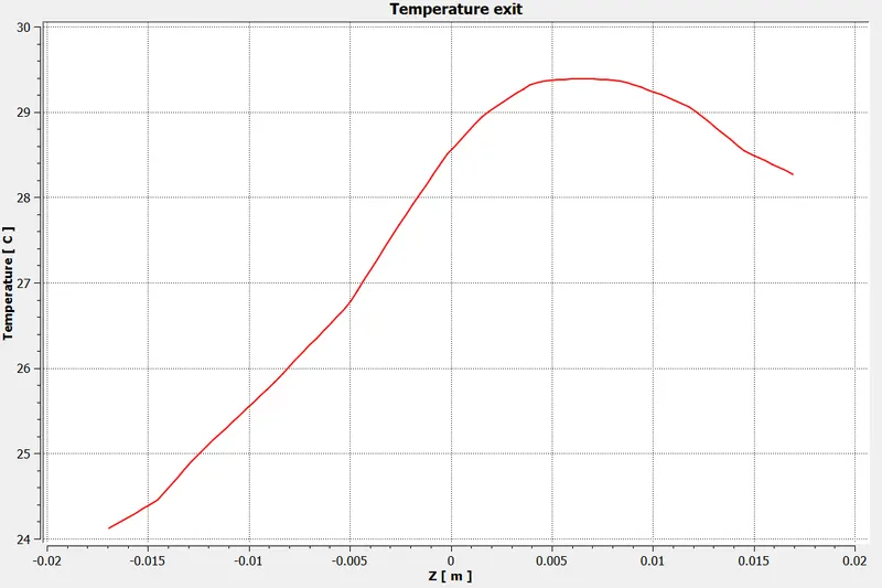
TEMPERATURE PLOTS:

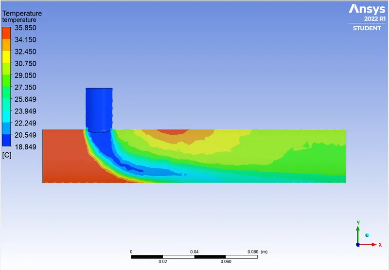
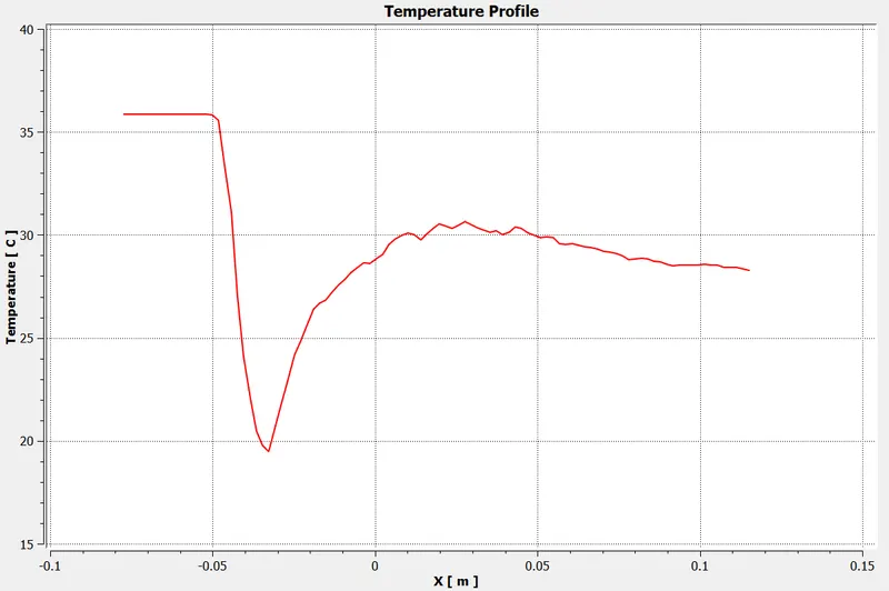
Along length:

Mid:

Exit:

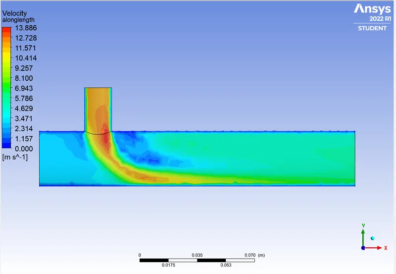
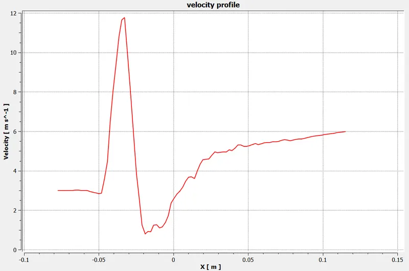
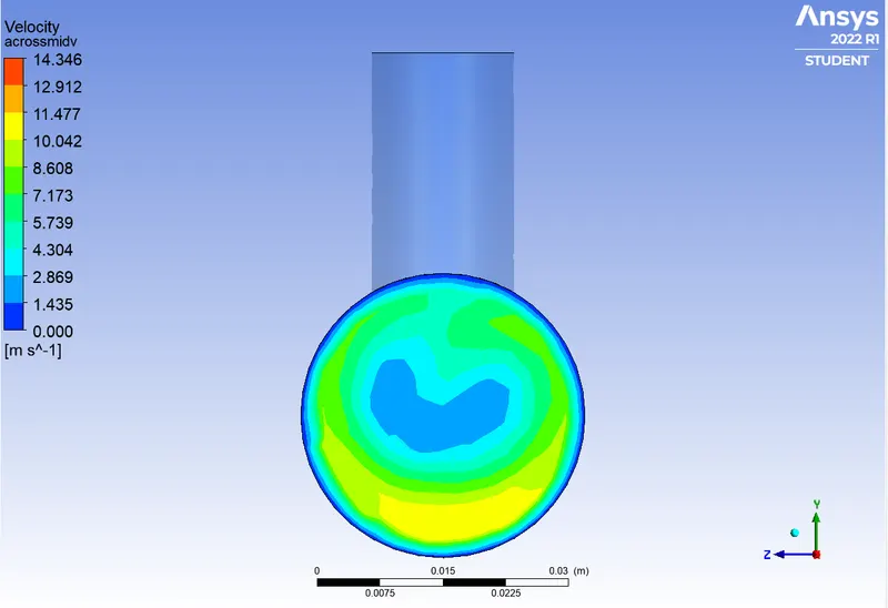
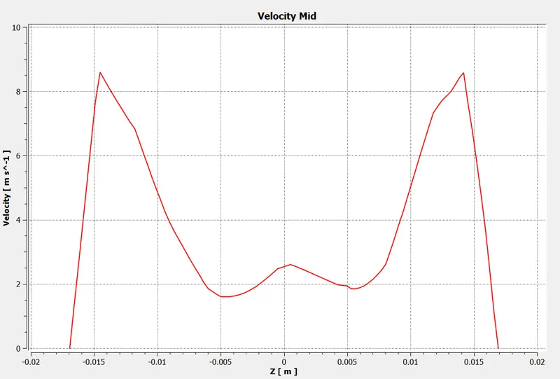
VELOCITY PLOTS:

Along Length:

Mid:

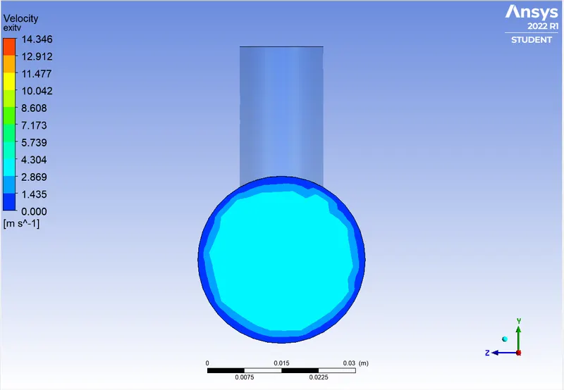
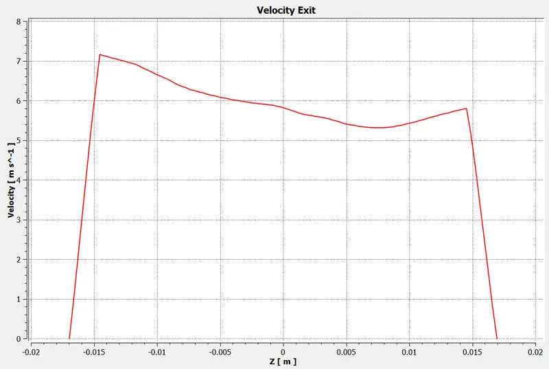
Exit:

CONCLUSION:

As evident from the results, A longer tee does not provide better performance than the short one; comparing the two cases:

CASE	Cell Count	Iterations	Avg. Outlet Temperature
1 (short tee)	14249	60	`27.38^o C`
2 (long tee)	39792	60	`27.52^o C`

Even the avg. outlet temperature is higher, although the difference is negligible. With a momentum ratio of 2, the avg. outlet temperature was even higher, approximately `30^o C`. Thus, a longer tee is not suggested based on the simulation.

Further, even the temperature profile near the exit is not as homogeneous as the shorter tee. Thus, Making the longer tee inefficient in mixing.