Week 3.5 - Deriving 4th order approximation of a 2nd order derivative using Taylor Table method

We are to calculate fourth-order approximation for f'' using central, left-skewed and right-skewed differencing methods.

We know that:

`f_i^q = (af_alpha + bf_beta ...+nf_lambda)/(Deltax^q) + O(Deltax^p) - - - - - - (i)`

here, `p` = order of accuracy and `q` = order of differentiation

CENTRAL-DIFFERENCE SCHEME:

We are to derive fourth-order accurate schemes of approximation, therefore:

`p = 4 ; q = 2`

We also know that for central scheme: `n = p + q - 1` where, `n` = number of nodes on stencil.

`therefore, n = 4 + 2 - 1 = 5`

hence, we will consider a 5 node stencil:

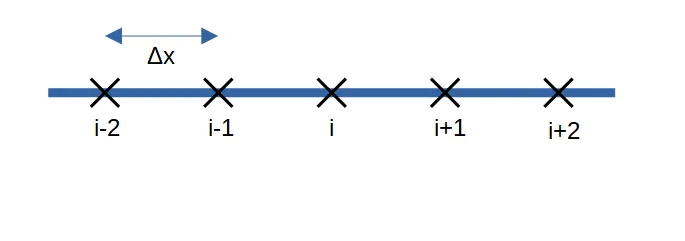
Substituting these values in our `eq.(i)` we get:

`Deltax^2(del^2y)/(delx^2) = af_(i-2) +bf_(i-1) +cf_i + df_(i+1) + ef_(i+2) + O(Deltax^6)------(ii)`

Populating Taylor Table according to this equation:

Stencil	`f(x)`	`Deltaxf`'`(x)`	`Deltax^2f`''`(x)`	`Deltax^3f`'''`(x)`	`Deltax^4f`''''`(x)`
`af_(i-2)`	`a`	`-2a`	`(4a)/2`	`-(8a)/6`	`(16a)/24`
`bf_(i-1)`	`b`	`-b`	`b/2`	`-b/6`	`b/24`
`cf_i`	`c`	`0`	`0`	`0`	`0`
`df_(i+1)`	`d`	`d`	`d/2`	`d/6`	`d/24`
`ef_(i+2)`	`e`	`2e`	`(4e)/2`	`(8e)/6`	`(16a)/24`
`Deltax^2(del^2y)/(delx^2)`	`0`	`0`	`1`	`0`	`0`

Since we only desire `f`'', therefore, the coefficient for all other Taylor Series terms must be zero. This gives us 5 equations corresponding to each column of the Taylor table.

We will write a Matlab function to solve this system of equations using the Matrix Inversion Method:

[Coefficient Matrix] x [Variable Matrix] = [Constant Matrix]

MATLAB gives us the values of coefficients:

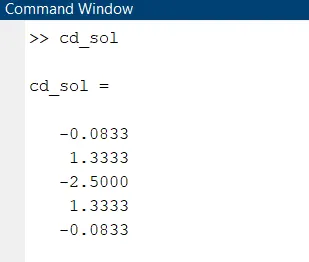
Substituting the values of co-efficient in `eq.(ii)`:

`Deltax^2(del^2y)/(delx^2) = -0.0833f_(i-2) +1.3333f_(i-1) -2.5f_i + 1.3333f_(i+1) -0.0833f_(i+2) + O(Deltax^6)`

Dividing both sides by `Deltax^2` we get:

`(del^2y)/(delx^2) = (-0.0833f_(i-2) +1.3333f_(i-1) -2.5f_i + 1.3333f_(i+1) + -0.0833f_(i+2))/(Deltax^2) + O(Deltax^4)`

This is the required Central-Differencing Scheme, the term `O(Deltax^4)` indicates that it is fourth-order accurate.

LEFT-SKEWED DIFFERENCE SCHEME:

For Skewed schemes, the number of minimum nodes required for accurate approximation is given as:

``n = p +q implies 4 +2 implies 6`

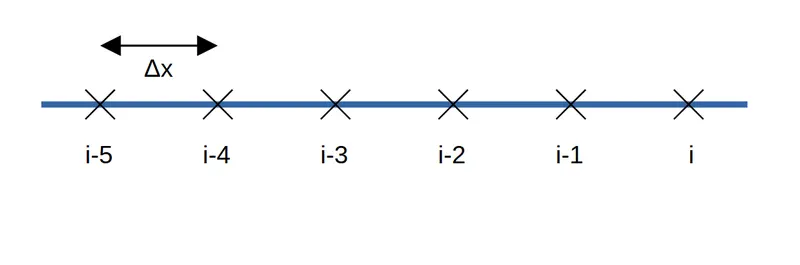
The minimum nodes required therefore are 6 for both Left and Right Skewed scheme. Substituting these values in `eq.(i)`:

`Deltax^2(del^2y)/(delx^2) = af_(i-5) + bf_(i-4) +cf_(i-3) +df_(i-2) + ef_(i-1) + gf_(i) + O(Deltax^6)------(iii)`

Expanding the individual terms and Populating Taylor table accordingly:

Stencil	`f(x)`	`Deltaxf`'`(x)`	`Deltax^2f`''`(x)`	`Deltax^3f`'''`(x)`	`Deltax^4f`''''`(x)`	`Deltax^5f`v`(x)`
`af_(i-5)`	`a`	`-5a`	`(25a)/2`	`-(125a)/6`	`(625a)/24`	`-(3125a)/120`
`bf_(i-4)`	`b`	`-4b`	`(16b)/2`	`-(64b)/6`	`(256b)/24`	`-(1024b)/120`
`cf_(i-3)`	`c`	`-3c`	`(9c)/2`	`-(27c)/6`	`(81c)/24`	`(-243c)/120`
`df_(i-2)`	`d`	`-2d`	`(4d)/2`	`-(8d)/6`	`(16d)/24`	`(-32d)/120`
`ef_(i-1)`	`e`	`-e`	`e/2`	`-e/6`	`e/24`	`-e/120`
`gf_(i)`	`g`	`0`	`0`	`0`	`0`	`0`
`(del^2y)/(delx^2)`	`0`	`0`	`1`	`0`	`0`	`0`

Solving for coefficients using Matrix Inversion Method:

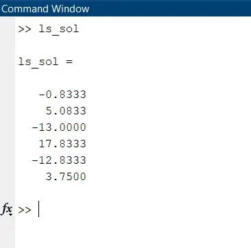
Substituting the values of coefficients in `eq.(iii)` we get:

`Deltax^2(del^2y)/(delx^2) = (-0.8333)f_(i-5) + (5.0833)f_(i-4) +(-13.0)f_(i-3) +(17.8333)f_(i-2) + (-12.8333)f_(i-1) + (3.75)f_(i) + O(Deltax^6)`

Dividing both sides by `Deltax^2`:

`(del^2y)/(delx^2) = (-(0.8333)f_(i-5) + (5.0833)f_(i-4) -(13.0)f_(i-3) +(17.8333)f_(i-2) -(12.8333)f_(i-1) + (3.75)f_(i))/(Deltax^2) + O(Deltax^4)`

Which is the required Left-Skewed Difference scheme, The term `O(Deltax^4)` indicates that it is fourth-order accurate.

RIGHT-SKEWED DIFFERENCE:

For Right-skewed difference, the nodes are positioned as the figure below:

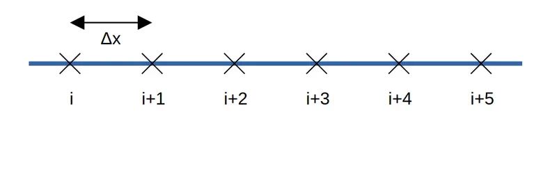
from `eq.(i)`, `Deltax^2(del^2y)/(delx^2) = af_(i+5) + bf_(i+4) +cf_(i+3) +df_(i+2) + ef_(i+1) + gf_(i) + O(Deltax^6)------(iv)`

Populating the Taylor table accordingly:

Stencil	`f(x)`	`Deltaxf`'`(x)`	`Deltax^2f`''`(x)`	`Deltax^3f`'''`(x)`	`Deltax^4f`''''`(x)`	`Deltax^5f`v`(x)`
`af_(i+5)`	`a`	`5a`	`(25a)/2`	`(125a)/6`	`(625a)/24`	`(3125a)/120`
`bf_(i+4)`	`b`	`4b`	`(16b)/2`	`(64b)/6`	`(256b)/24`	`(1024b)/120`
`cf_(i+3)`	`c`	`3c`	`(9c)/2`	`(27c)/6`	`(81c)/24`	`(243c)/120`
`df_(i+2)`	`d`	`2d`	`(4d)/2`	`(8d)/6`	`(16d)/24`	`(32d)/120`
`ef_(i+1)`	`e`	`e`	`e/2`	`e/6`	`e/24`	`e/120`
`gf_(i)`	`g`	`0`	`0`	`0`	`0`	`0`
`(del^2y)/(delx^2)`	`0`	`0`	`1`	`0`	`0`	`0`

On Solving using Matrix Inversion Method:

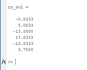
Substituting the values of coefficients in `eq.(iv)` we get:

`Deltax^2(del^2y)/(delx^2) = (-0.8333)f_(i-5) + (5.0833)f_(i-4) +(-13.0)f_(i-3) +(17.8333)f_(i-2) + (-12.8333)f_(i-1) + (3.75)f_(i) + O(Deltax^6)`

Dividing both sides by `Deltax^2`:

`(del^2y)/(delx^2) = (-(0.8333)f_(i-5) + (5.0833)f_(i-4) -(13.0)f_(i-3) +(17.8333)f_(i-2) -(12.8333)f_(i-1) + (3.75)f_(i))/(Deltax^2) + O(Deltax^4)`

Which is the required Right-Skewed Difference scheme, The term `O(Deltax^4)` indicates that it is fourth-order accurate.

CENTRAL-DIFFERENCE FUNCTION:

function [sol, error] = cd_table(a,b,x,dx, analytical)
 
% Using Matrix Inversion Method
sol=inv(a)*b;

% Central-Difference Derivative

approx = (sol(1).*(exp(x-(2*dx)).*cos(x-(2*dx)))+sol(2).*(exp(x-dx).*cos(x-dx))+sol(3).*(exp(x).*cos(x))+sol(4).*(exp(x+dx).*cos(x+dx))+sol(5).*(exp(x+(2*dx)).*cos(x+(2*dx))))./(dx.^2);

% Error
error = abs(analytical -approx);

end

RIGHT-SKEWED DIFFERENCE FUNCTION:

function [sol,error] = rs_table(a,b,x,dx, analytical)
 
% Using Matrix Inversion Method
sol=inv(a)*b;

% Right-Skewed Derivative
approx = (sol(1).*(exp(x+(5*dx)).*cos(x+(5*dx)))+sol(2).*(exp(x+(4*dx)).*cos(x+(4*dx)))+sol(3).*(exp(x+(3*dx)).*cos(x+(3*dx)))+sol(4).*(exp(x+(2*dx)).*cos(x+(2*dx)))+sol(5).*(exp(x+dx).*cos(x+dx))+sol(6).*(exp(x).*cos(x)))./(dx.^2);

% Error
error = abs(analytical -approx);

end

LEFT-SKEWED DIFFERENCE FUNCTION:

function [sol,error] = ls_table(a,b,x,dx, analytical)
 
% Using Matrix Inversion Method
sol=inv(a)*b;

% Left-Skewed Derivative
approx = (sol(1).*(exp(x-(5*dx)).*cos(x-(5*dx)))+sol(2).*(exp(x-(4*dx)).*cos(x-(4*dx)))+sol(3).*(exp(x-(3*dx)).*cos(x-(3*dx)))+sol(4).*(exp(x-(2*dx)).*cos(x-(2*dx)))+sol(5).*(exp(x-dx).*cos(x-dx))+sol(6).*(exp(x).*cos(x)))./(dx.^2);

% Error
error = abs(analytical - approx);

end

MAIN SCRIPT

close all
clear all
clc

% Pre-Requisite
% Given function = exp(x)*cos(x)
x = pi/3;
dx = linspace(pi/100,pi/500,100);


% Analytical Derivative of exp(x)*cos(x) = -2*(exp(x)*sin(x))
analytical = -2*exp(x)*sin(x);

% Matrices for Central Difference
% Constant Matrix
b = [0;0;1;0;0];
% Coefficient Matrix
cd_a = [1 1 1 1 1 ; -2 -1 0 1 2; 4/2 1/2 0 1/2 4/2; -(8/6) -(1/6) 0 1/6 8/6; 16/24 1/24 0 1/24 16/24];

% Calculate the value of the variables and error
[cd_sol,cd_error] = cd_table(cd_a,b,x,dx,analytical);

% Matrices for Left-Skewed Scheme
% Constant Matrix
b_skew = [0;0;1;0;0;0];
% Coefficient Matrix
ls_a = [1 1 1 1 1 1;-5 -4 -3 -2 -1 0;25/2 16/2 9/2 4/2 1/2 0;-(125/6) -(64/6) -(27/6) -(8/6) -(1/6) 0;625/24 256/24 81/24 16/24 1/24 0;-(3125/120) -(1024/120) -(243/120) -(32/120) -(1/120) 0];

% Calculate the value of the variables and error
[ls_sol,ls_error] = ls_table(ls_a,b_skew,x,dx,analytical);

% Matrices for Right-Skewed Scheme
% Coefficient Matrix
rs_a = [1 1 1 1 1 1;5 4 3 2 1 0;25/2 16/2 9/2 4/2 1/2 0;(125/6) (64/6) (27/6) (8/6) (1/6) 0;625/24 256/24 81/24 16/24 1/24 0;(3125/120) (1024/120) (243/120) (32/120) (1/120) 0];

% Calculate the value of the variables and error
[rs_sol,rs_error] = rs_table(rs_a,b_skew,x,dx,analytical);

figure('Name','Comparison of Centered and Skewed Differencing Schemes')
loglog(dx, cd_error,'black','DisplayName','Central Difference');
hold on
loglog(dx, rs_error,'cyan','DisplayName','Right-Skewed Difference');
hold on
loglog(dx, ls_error,'magenta','DisplayName','Left-Skewed Difference')
legend show
xlabel('\Deltax')
ylabel('Error b/w actual and numerical value')

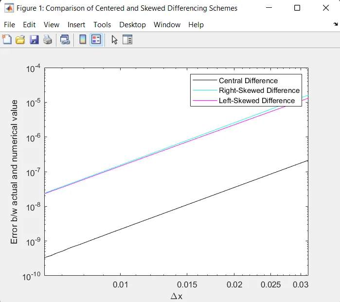
PLOT:

CONCLUSION:

• We can observe that for any value of `Deltax`, the Centered Difference Scheme has the lowest error, making it the most accurate method. Right-Skewed and Left-Skewed schemes have almost similar accuracy.
• As we increase `Deltax`, the error increases, implying that for most accurate results `Deltax` should be kept as small.

SIGNIFICANCE OF SKEWED SCHEMES:

Although less accurate, Skewed Schemes shine in certain use cases. They are extremely helpful in determining the values at boundaries where central-differencing cannot be applied. SInce at the boundaries nodes are concentrated only at one side and thus applying central-differencing is not possible since it needs nodes on both sides of the point where the value is to be calculated.