Week 5.1 - Mid term project - Solving the steady and unsteady 2D heat conduction problem
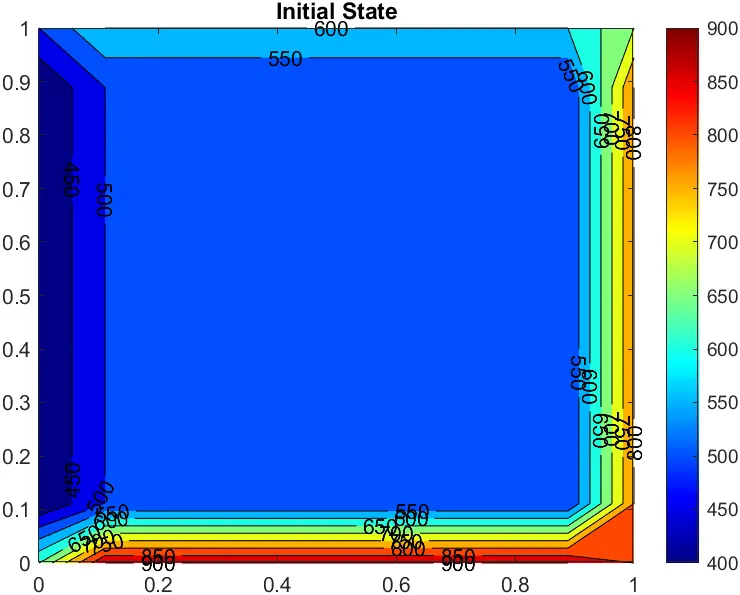
We will be using iterative point techniques to solve the 2D Heat-Conduction Equation for this exercise. We have the following Boundary Conditions:
Top Boundary(`T_T`) = 600 K
Bottom Boundary(`T_B`) = 900 K
Left Boundary(`T_L`) = 400 K
Right Boundary(`T_R`) = 800 K
and we will assume the initial temperature to be 500K.
We will be using Jacobi Method, Gauss-Seidel Method and Successive Over-Relaxation Method to calculate the temperature at our Point, i.e. `T_P`, using both Steady and Transient state analysis.
Initial Plot:
FOR STEADY STATE:
`(del^2T)/(delx^2) + (del^2T)/(dely^2) = 0-----(i)`
Discretizing `eq.(i)`:
`T_P = (1/k)*[(T_L +T_R)/(Deltax^2) + (T_P + T_B)/(Deltay^2)]-----(ii)`
where, `k = 2(Deltax^2+Deltay^2)/(Deltax^2Deltay^2)`
Main Function:
close all
clear all
clc

% Pre-Requisites
nx = 10; %number of nodes along x-axis
ny = nx; %number of nodes along y-axis

% let domain be a unit square, discretising:
x = linspace(0,1,nx);
y = x ;
dx = x(2) - x(1);
dy = dx;
k = 2*((dx^2)+(dy^2))/((dx^2)*(dy^2));

% Initial Condition
init = 500;
T = init*ones(nx,ny);

% Boundary Conditions
Tt  = 600;
Tb = 900;
Tl = 400;
Tr = 800;
T(1,:) = Tt;
T(ny,:) = Tb;
T(:,1) = Tl;
T(:,nx) = Tr;

% Corners
T(1,1) = (Tt+Tl)/2;
T(1,nx) = (Tt+Tr)/2;
T(ny,1) = (Tb+Tl)/2;
T(nx,ny) = (Tb+Tr)/2;

% Calling Solver Functions
gauss_seidel(x,y,dx,dy,T,nx,ny,k);
jacobi(x,y,dx,dy,T,nx,ny,k);
sor(x,y,dx,dy,T,nx,ny,k);
JACOBI METHOD:
Applying Jacobi Method on `eq.(ii)`:
`T_(i,j) = (1/k)*[(T_(i,j-1)^(old) +T_(i,j+1)^(old))/(Deltax^2) + (T_(i-1,j)^(old)+T_(i+1,j)^(old))/(Deltay^2)]`
where, `i` denotes abscissa and `j` denotes ordinate of our domain grid.
Jacobi Function:
function jacobi(x,y,dx,dy,T,nx,ny,k)
Told = T;
tolerance = 1e-4;
error = 10;
iter = 0;

while(error>tolerance)
    iter = iter+1;
    for i=2:ny-1
        for j=2:nx-1
            term1 = (Told(i,j-1)+Told(i,j+1))/(dx^2);
            term2 = (Told(i-1,j)+Told(i+1,j))/(dy^2);
            T(i,j) =  (1/k)*((term1)+(term2));
        end
    end
    error = max(max(abs(T-Told)));
    Told = T;
    figure(1)
    contourf(x,y,flipud(T),'ShowText','on')
    colormap(jet)
    colorbar
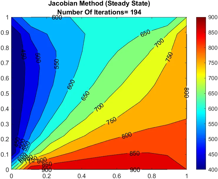
    title(sprintf('Jacobian Method (Steady State)\nNumber Of Iterations= %d',iter))
    pause(0.005)
end
Jacobi Plot:
GAUSS-SEIDEL METHOD:
Applying Gauss-Seidel Method on `eq.(ii)`:
`T_(i,j) = (1/k)*[(T_(i,j-1) +T_(i,j+1))/(Deltax^2) + (T_(i-1,j)+T_(i+1,j))/(Deltay^2)]`
Gauss-Seidel Function:
function gauss_seidel(x,y,dx,dy,T,nx,ny,k)
Told = T;
tolerance = 1e-4;
error = 10;
iter = 0;

while(error>tolerance)
    iter = iter+1;
    for i=2:ny-1
        for j=2:nx-1
            term1 = (T(i,j-1)+T(i,j+1))/(dx^2);
            term2 = (T(i-1,j)+T(i+1,j))/(dy^2);
            T(i,j) =  (1/k)*((term1)+(term2));
        end
    end
    error = max(max(abs(T-Told)));
    Told = T;
    figure(2)
    contourf(x,y,flipud(T),'ShowText','on')
    colormap(jet)
    colorbar
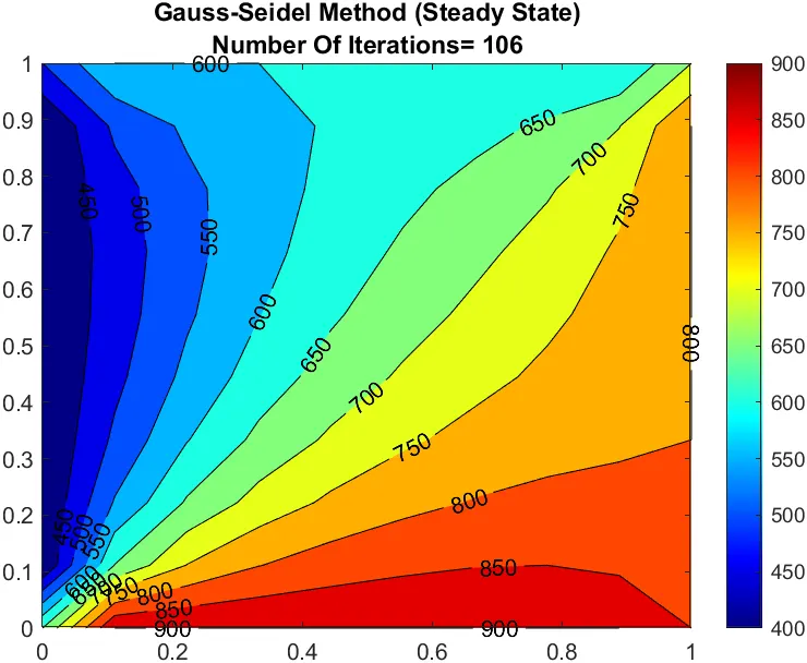
    title(sprintf('Gauss-Seidel Method (Steady State)\nNumber Of Iterations= %d',iter))
    pause(0.005)
end
Gauss-Seidel Plot:
SUCCESSIVE-OVER RELAXATION METHOD (SOR):
SOR method is given as:
`T_(i,j) = (1-omega)*(T_(i,j)^(old))+ omega*(T_(i,j)^(GS))`
where, `T_(i,j)^(GS)` is `T_(i,j)` calculated using Gauss-Seidel Method, and `omega` is relaxation factor.
Usually, `omega` lies between `0` and `2`, and if `omega = 1`, the `T_(i,j)^(SOR) = T_(i,j)^(GS)`.
SOR Function:
function sor(x,y,dx,dy,T,nx,ny,k)
Told = T;
tolerance = 1e-4;
error = 10;
iter = 0;
omega = 1.3;

while(error>tolerance)
    iter = iter+1;
    for i=2:ny-1
        for j=2:nx-1
            term1 = (T(i,j-1)+T(i,j+1))/(dx^2);
            term2 = (T(i-1,j)+T(i+1,j))/(dy^2);
            term3 = (1/k)*((term1)+(term2));
            T(i,j) =  (1-omega)*T(i,j) + omega*term3;
        end
    end
    error = max(max(abs(T-Told)));
    Told = T;
    figure(3)
    contourf(x,y,flipud(T),'ShowText','on')
    colormap(jet)
    colorbar
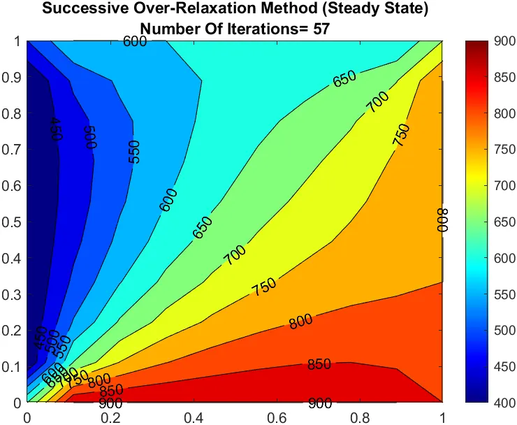
    title(sprintf('Successive Over-Relaxation Method (Steady State)\nNumber Of Iterations= %d',iter))
    pause(0.005)
end
SOR Plot:
FOR TRANSIENT STATE:
For transient state the 2D Heat Conduction Equation is given as:
`(delT)/(delt)= alpha*[(del^2T)/(delx^2) + (del^2T)/(dely^2)]---------(iii)`
Discretizing `eq.(iii)` implicitly:
`(T_p^(n+1) - T_p^n)/(Deltat) = alpha*[(T_L - 2*(T_p) + T_R)/(Deltax^2) +(T_T - 2*(T_p) + T_B)/(Deltay^2)]^(n+1)`
We can further simplify it as:
`T_p^(n+1) = (1/(1+k1+k2))*[T_p^n + k1(T_L + T_R)^(n+1) + k2(T_T + T_B)^(n+1)]-----(iv)`
Where, `k1 = alpha(Deltat)/(Deltax^2), k2 = alpha(Deltat)/(Deltay^2)`;
`alpha = `Thermal Diffusivity of Material
Main Function:
close all
clear all
clc

% Pre-Requisites
nx = 10; %number of nodes along x-axis
ny = nx; %number of nodes along y-axis
alpha = 1.5; %thermal diffusivity

% let domain be a unit square, discretising:
x = linspace(0,1,nx);
y = x ;
dx = x(2) - x(1);
dy = dx;
dt = 1e-2;
k1 = alpha*(dt/dx^2);
k2 = alpha*(dt/dy^2);

% Initial Condition
init = 500;
T = init*ones(nx,ny);

% Boundary Conditions
Tt  = 600;
Tb = 900;
Tl = 400;
Tr = 800;
T(1,:) = Tt;
T(ny,:) = Tb;
T(:,1) = Tl;
T(:,nx) = Tr;

% Corners
T(1,1) = (Tt+Tl)/2;
T(1,nx) = (Tt+Tr)/2;
T(ny,1) = (Tb+Tl)/2;
T(nx,ny) = (Tb+Tr)/2;

% Caling Solver Functions
transient_gauss_seidel(x,y,T,nx,ny,k1,k2);
transient_jacobi(x,y,T,nx,ny,k1,k2);
transient_sor(x,y,T,nx,ny,k1,k2);
JACOBI METHOD:
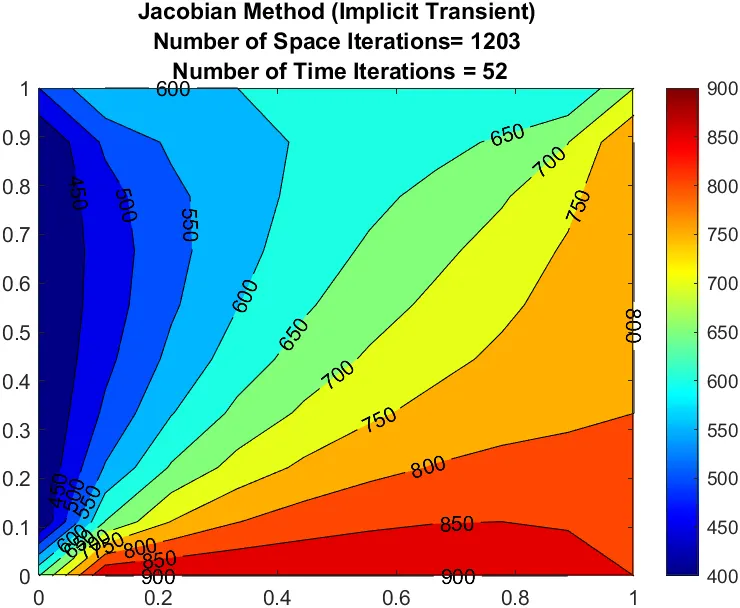
Applying Jacobi method on `eq.(iv)`:
`T_(i,j)^(Next) = (1/(1+k1+k2))*[T_(i,j)^(prev) + k1(T_(i,j-1)^(old) + T_(i,j+1)^(old))^(Next) + k2(T_(i-1,j)^(old) + T_(i,j+1)^(old))^(Next)]`
where, `prev` is the previous node point and `Next` is the node point we are calculating.
Jacobi Function:
function transient_jacobi(x,y,T,nx,ny,k1,k2)
Told = T;
Tprev = T;
tolerance = 1e-4;
iter = 0;
t_iter = 0;
convergence = 10;

while(convergence>tolerance)
    t_iter = t_iter +1;
    error = 10;
    while(error>tolerance)
        iter = iter+1;
        for i=2:ny-1
            for j=2:nx-1
                term1 = (Told(i,j-1)+Told(i,j+1))*k1;
                term2 = (Told(i-1,j)+Told(i+1,j))*k2;
                T(i,j) =  (1/(1+(2*(k1+k2))))*(Tprev(i,j)+(term1)+(term2));
            end
        end
        error = max(max(abs(T-Told)));
        Told = T;
        figure(1)
        contourf(x,y,flipud(T),'ShowText','on')
        colormap(jet)
        colorbar
        title(sprintf('Jacobian Method (Implicit Transient)\nNumber of Space Iterations= %d\n Number of Time Iterations = %d',iter,t_iter))
        pause(0.005)
    end
    convergence = max(max(abs(T- Tprev)));
    Tprev = T;
end
Jacobi Plot:
GAUSS-SEIDEL METHOD:
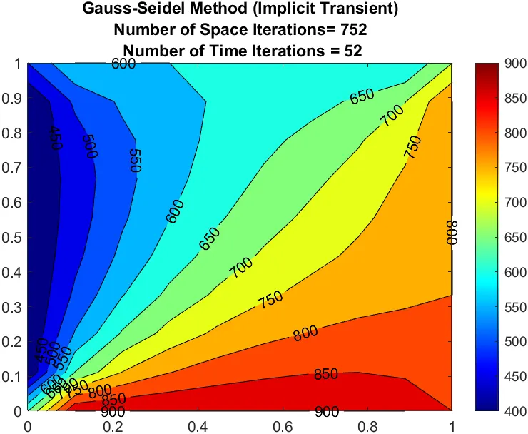
Applying Gauss-Seidel method on `eq.(iv)`:
`T_(i,j)^(Next) = (1/(1+k1+k2))*[T_(i,j)^(prev) + k1(T_(i,j-1) + T_(i,j+1))^(Next) + k2(T_(i-1,j) + T_(i,j+1))^(Next)]`
Gauss-Seidel Function:
function transient_gauss_seidel(x,y,T,nx,ny,k1,k2)
Told = T;
Tprev = T;
tolerance = 1e-4;
iter = 0;
t_iter = 0;
convergence = 10;

while(convergence>tolerance)
    t_iter = t_iter +1;
    error = 10;
    while(error>tolerance)
        iter = iter+1;
        for i=2:ny-1
            for j=2:nx-1
                term1 = (T(i,j-1)+T(i,j+1))*k1;
                term2 = (T(i-1,j)+T(i+1,j))*k2;
                T(i,j) =  (1/(1+(2*(k1+k2))))*(Tprev(i,j)+(term1)+(term2));
            end
        end
        error = max(max(abs(T-Told)));
        Told = T;
        figure(2)
        contourf(x,y,flipud(T),'ShowText','on')
        colormap(jet)
        colorbar
        title(sprintf('Gauss-Seidel Method (Implicit Transient)\nNumber of Space Iterations= %d\n Number of Time Iterations = %d',iter,t_iter))
        pause(0.005)
    end
    convergence = max(max(abs(T- Tprev)));
    Tprev = T;
end
Gauss-Seidel Plot:
SUCCESSIVE OVER-RELAXATION(SOR) METHOD:
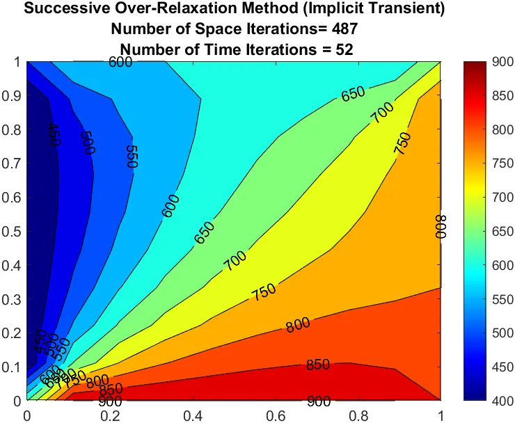
SOR method depends on Gauss-Seidel, so it's the same as for steady-state since the necessary changes have already been applied to the Gauss-Seidel method.
`T_(i,j) = (1-omega)*(T_(i,j)^(old))+ omega*(T_(i,j)^(GS))`
SOR function:
function transient_sor(x,y,T,nx,ny,k1,k2)

Told = T;
Tprev = T;
tolerance = 1e-4;
iter = 0;
t_iter = 0;
omega = 1.3;
convergence = 10;

while(convergence>tolerance)
    error = 10;
    t_iter = t_iter +1;
    while(error>tolerance)
        iter = iter+1;
        for i=2:ny-1
            for j=2:nx-1
                term1 = (T(i,j-1)+T(i,j+1))*k1;
                term2 = (T(i-1,j)+T(i+1,j))*k2;
                term3 =  (1/(1+(2*(k1+k2))))*(Tprev(i,j)+(term1)+(term2));
                T(i,j) =  (1-omega)*T(i,j) + omega*term3;
            end
        end
        error = max(max(abs(T-Told)));
        Told = T;
        figure(3)
        contourf(x,y,flipud(T),'ShowText','on')
        colormap(jet)
        colorbar
        title(sprintf('Successive Over-Relaxation Method (Implicit Transient)\nNumber of Space Iterations= %d\n Number of Time Iterations = %d',iter,t_iter))
        pause(0.005)
    end
    convergence = max(max(abs(T- Tprev)));
    Tprev = T;
end
SOR Plot:
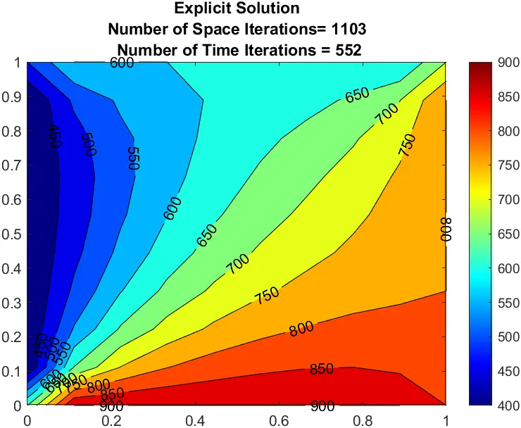
For Explicit Solution, `eq.(iii)` becomes:
`(T_p^(n+1) - T_p^n)/(Deltat) = alpha*[(T_L - 2*(T_p) + T_R)/(Deltax^2) +(T_T - 2*(T_p) + T_B)/(Deltay^2)]^n`
on further simplification:
`T_(i,j) = T_(i,j)^(prev)*(1-2*(k1+k2))+k1*(T_(i,j-1)^(prev) +T_(i,j+1)^(prev))+k2*(T_(i-1,j)^(prev) + T_(i+1,j)^(prev))`
Explicit Program:
close all
clear all
clc

% Pre-Requisites
nx = 10; %number of nodes along x-axis
ny = nx; %number of nodes along y-axis
alpha = 0.1; %thermal diffusivity

% let domain be a unit square, discretising:
x = linspace(0,1,nx);
y = x;
dx = x(2) - x(1);
dy = dx;
dt = 1e-2;
k1 = alpha*(dt/dx^2);
k2 = alpha*(dt/dy^2);
cfl = k1+k2;

% Initial Condition
init = 500;
T = init*ones(nx,ny);

% Boundary Conditions
Tt  = 600;
Tb = 900;
Tl = 400;
Tr = 800;
T(1,:) = Tt;
T(ny,:) = Tb;
T(:,1) = Tl;
T(:,nx) = Tr;

% Corners
T(1,1) = (Tt+Tl)/2;
T(1,nx) = (Tt+Tr)/2;
T(ny,1) = (Tb+Tl)/2;
T(nx,ny) = (Tb+Tr)/2;

% Initialisation
Told = T;
Tprev = T;
tolerance = 1e-4;
iter = 0;
t_iter = 0;
convergence = 10;

% Solution
while(convergence>tolerance)
    t_iter = t_iter +1;
    error = 10;
    while(error>tolerance)
        iter = iter+1;
        for i=2:ny-1
            for j=2:nx-1
                term1 = (Tprev(i,j-1)+Tprev(i,j+1))*k1;
                term2 = (Tprev(i-1,j)+Tprev(i+1,j))*k2;
                T(i,j) =  ((1-(2*(k1+k2)))*(Tprev(i,j)))+(term1)+(term2);
            end
        end
        error = max(max(abs(T-Told)));
        Told = T;
        figure(1)
        contourf(x,y,flipud(T),'ShowText','on')
        colormap(jet)
        colorbar
        title(sprintf('Explicit Solution\nNumber of Space Iterations= %d\n Number of Time Iterations = %d',iter,t_iter))
        pause(0.005)
    end
    convergence = max(max(abs(T- Tprev)));
    Tprev = T;
end
Explicit Plot:
CONCLUSION:
- As we see, irrespective of solving for steady state or transient state, the rate of convergenge follows the following trend: SOR > Gauss-Seidel > Jacobi , making SOR most efficient solver.
- The CFL condition as discussed in previous challenge is `C_max <=1`, for explicit solutions, whereas implicit solutions can tolerate high values of `C_max`.
- This is why, Explicit method has unusually high number of iterations, since reducing `C_max` always results in calculation for more nodepoints or reduction of alpha.