Week 7 - Simulation of a 1D Super-sonic nozzle flow simulation using Macormack Method

Aim:

To simulate the isentropic flow through the (quasi 1D subsonic and supersonic nozzle) convergent Divergent nozzle.

Introduction:

The flow at the inlet of the nozzle comes from the reservoir, which has a large area and hence velocity is small. Since the velocity is nearly zero, therefore P₀ and T₀ are the stagnation pressure and temperatures respectively at the inlet. The primitive variables at the throat have represented a superscript (*) and the exit variables are denoted with a subscript (e).

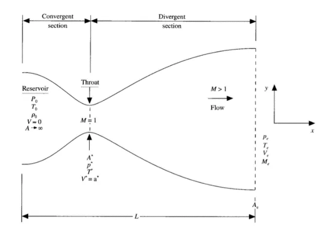
Ideally, the flow enters subsonic at the inlet from reservoir, reaches Mach=1 at the throat for a critical exit pressure, leaving supersonic flow at the end of the divergent section. If the exit static pressure is more than the critical pressure it leads to shocks (Normal shocks, oblique shocks).

For the given condition, we don’t discuss about the shocks which means the flow is supersonic at the outlet.

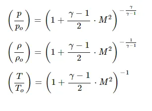
We use some of the compressible flow relations for calculating the exact values.

MacCormack method:

In computational fluid dynamics, the MacCormack method is a widely used discretization scheme for the numerical solution of hyperbolic partial differential equations.

MacCormack’s method provides second-order accuracy without the involvement of second-order derivatives thus reducing the complexity of the calculation. It is an explicit method. In the predictor step, the spatial derivatives of governing equations are replaced with forward differencing and in the corrector step, the spatial terms are replaced with the backward differencing.

Non conservation form:

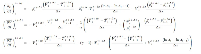
Predictor step:

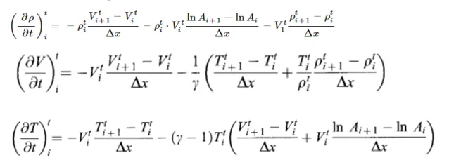
We get the predicted values of from the following equation:

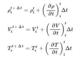
Non-conservation form:

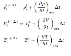
Corrector step

Average time derivatives are taken by

Conservation form:

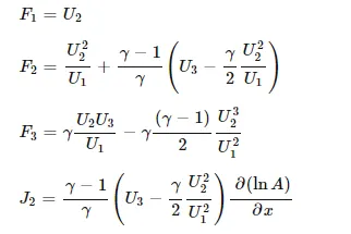
Let us define the elements of solution vector(U), the flux vector (F) and the source term (j) as follows,

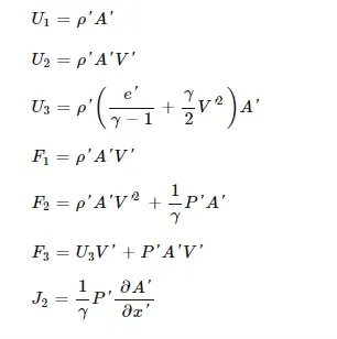
With these elements, the governing equation can be written as

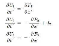
To obtain the primitive variables we must decode the elements U1, U2, U3 as follows

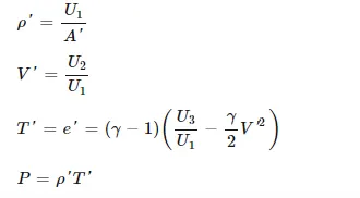
The pure form of the Flux terms,

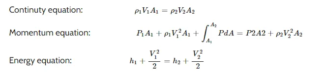
Governing equations:

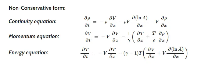
The governing continuity, momentum and energy equations are for this quasi-one-dimensional, steady, isentropic flow can be expressed, as respectively, as

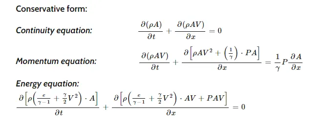
We solve the governing equations in two forms Conservation and non-conservation form.

Boundary condition:

Non-conservation form:

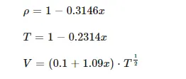
Initial conditions are specified as

Boundary conditions at the subsonic inflow

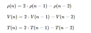
The boundary condition at supersonic outflow

Conservation form:

Let us assume the elements of the solution vector(U), the flux(F) and the source term(J) as follows,

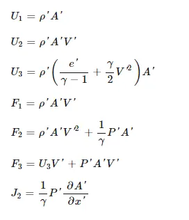
With these elements, the governing equation can be rewritten as

The pure form of the Flux terms,

The initial conditions at time t=0 give the values of primitive variables at the inlet. This provides values of F1, F2, and F3 which are functions of U1, U2 and U3.

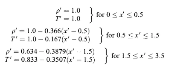
The boundary conditions for the subsonic-supersonic nozzle solution using the conservation form of the governing equations are theoretically same.

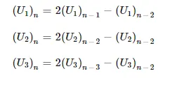
The flow properties downstream to the supersonic outflow are obtained by linear extrapolation from the two adjacent internal points. If n denotes the grid points at the outflow boundary, then

Main code:

%  Supersonic nozzle flow equation
clear all
close all
clc

% Defining Inputs

% length of the nozzle
L = 3;
% No.of grid points
n = 31;
% Defining Mesh
x = linspace(0,L,n);  
% Mesh Size 
dx = x(2)-x(1);  
% Throat 
throat = (n+1)/2;
% No.of iterations % Time steps
nt = 1400;
% Area
a = 1+2.2.*(x-1.5).^2;     
% Fluid properties
gamma = 1.4;
% CFL number
C = 0.5;                    

% Non-conservative form 
 [rho_Nc,v_Nc,T_Nc,P_Nc,M_Nc,Mass_flow_Nc] = NC_fcn(n,x,dx,gamma,throat,nt,a,C);
% Conservative form
 [rho_C,v_C,T_C,P_C,M_C,Mass_flow_C] = con_fcn(n,x,dx,gamma,throat,nt,a,C);

% Comparison of steady state results, Conservative & Non-conservative results
Terms = [{'N.D density'};{'N.D tempearture'};{'N.D pressure'};{'Mach number'};{'N.D velocity'}];
Exact_Sol = [0.634;0.833;0.528;1;1];
Non_conservative_Sol = [rho_Nc(throat);T_Nc(throat);P_Nc(throat);M_Nc(throat);v_Nc(throat)];
Conservative_Sol = [rho_C(throat);T_C(throat);P_C(throat);M_C(throat);v_C(throat)];
table(Terms,Exact_Sol,Non_conservative_Sol,Conservative_Sol)

% Comparison of Normalized mass flow rate distributions of Non_conservative form & Conservative form
figure(7)
plot(x,Mass_flow_Nc)
hold on
plot(x,Mass_flow_C)
xlabel('length of nozzle')
ylabel('mass flow rate')
legend('Non-conservative form','Conservative from')
title('Comparison mass flow distributions of Non-conservative form & Conservative from')
grid on

Non-conservation function code:

function [rho_Nc,v_Nc,T_Nc,P_Nc,M_Nc,Mass_flow_Nc] = NC_fcn(n,x,dx,gamma,throat,nt,a,C)
                                                                
% Calculate initial profiles
rho_Nc = 1-0.31468*x;                     % Density
T_Nc = 1-0.2314*x;                        % Temperature
v_Nc = (0.1+1.09*x.*T_Nc.^0.5);           % Velocity

% Non-conservative form of Supersonic nozzle flow equation
% Maccormack method
    % Outer loop
    tic
for k=1:nt
    % Predictor step
%     % Creating copy
    rho_old = rho_Nc;
    v_old = v_Nc;
    T_old = T_Nc;
    dt = min(C.*dx./(sqrt(T_Nc)+v_Nc));
    for j=2:n-1
         % derivatives
        dv_dx = (v_Nc(j+1)-v_Nc(j))/dx;
        drho_dx = (rho_Nc(j+1)-rho_Nc(j))/dx;
        dT_dx = (T_Nc(j+1)-T_Nc(j))/dx;
        dloga_dx = (log(a(j+1))-log(a(j)))/dx;
        
        % Continuty Equation
        drho_dt_p(j) = -rho_Nc(j)*dv_dx-rho_Nc(j)*v_Nc(j)*dloga_dx-v_Nc(j)*drho_dx;
       
        % Momentum Equation
        dv_dt_p(j) = -v_Nc(j)*dv_dx-(1/gamma)*(dT_dx+(T_Nc(j)/rho_Nc(j))*drho_dx); 
        
        % Energy Equation
        dT_dt_p(j) = -v_Nc(j)*dT_dx-(gamma-1)*T_Nc(j)*(dv_dx+v_Nc(j)*dloga_dx);
        
        % Solution update
        v_Nc(j) = v_Nc(j)+dv_dt_p(j)*dt;
        rho_Nc(j) = rho_Nc(j)+drho_dt_p(j)*dt;
        T_Nc(j) = T_Nc(j)+dT_dt_p(j)*dt;
      
    end
    
        % Corrector step
        
        for j=2:n-1
        % derivatives
        dv_dx = (v_Nc(j)-v_Nc(j-1))/dx;
        drho_dx = (rho_Nc(j)-rho_Nc(j-1))/dx;
        dT_dx = (T_Nc(j)-T_Nc(j-1))/dx;
        dloga_dx = (log(a(j))-log(a(j-1)))/dx;
        
        % Continuty Equation
        drho_dt_c(j) = -rho_Nc(j)*dv_dx-rho_Nc(j)*v_Nc(j)*dloga_dx-v_Nc(j)*drho_dx;
       
        % Momentum Equation
        dv_dt_c(j) = -v_Nc(j)*dv_dx-(1/gamma)*(dT_dx+(T_Nc(j)/rho_Nc(j))*drho_dx); 
        
        % Energy Equation
        dT_dt_c(j) = -v_Nc(j)*dT_dx-(gamma-1)*T_Nc(j)*(dv_dx+v_Nc(j)*dloga_dx);
        
        end
        % Compute the average time derivative 
        drho_dt = 0.5*(drho_dt_p+drho_dt_c);
        dv_dt = 0.5*(dv_dt_p+dv_dt_c);
        dT_dt = 0.5*(dT_dt_p+dT_dt_c);
        
        % Final solution update 
        for i = 2:n-1
            rho_Nc(i) = rho_old(i)+drho_dt(i)*dt;
            v_Nc(i) = v_old(i)+dv_dt(i)*dt;
            T_Nc(i) = T_old(i)+dT_dt(i)*dt;            
        end
        
        % Applying Boundry conditions
        % Inlet Boundry conditions
        v_Nc(1) = 2*v_Nc(2)-v_Nc(3); % Velocity
        % Outlet Boundry conditions
        v_Nc(n) = 2*v_Nc(n-1)-v_Nc(n-2);
        rho_Nc(n) = 2*rho_Nc(n-1)-rho_Nc(n-2);
        T_Nc(n) = 2*T_Nc(n-1)-T_Nc(n-2);
        
        % Calculating Pressure, Mach number & mass flow rate     
        P_Nc = rho_Nc.*T_Nc;                % Pressure
        M_Nc = v_Nc./(T_Nc.^(0.5));         % Mach number
        Mass_flow_Nc = rho_Nc.*v_Nc.*a;     % Mass flow rate
        
        % Capturing flow field values at throat for each time step
        rho_throat(k) = rho_Nc(throat);
        v_throat(k) = v_Nc(throat);
        T_throat(k) = T_Nc(throat);
        P_throat(k) = P_Nc(throat);
        M_throat(k) = M_Nc(throat);
        flow_rate_throat(k) = Mass_flow_Nc(throat);
        
        figure(1)
        % Variation of Mass flow rate distribution inside the nozzle at different time steps during the time-marching process
        if k==100
            plot(x,Mass_flow_Nc)
            hold on
        else if k==200
                plot(x,Mass_flow_Nc)
                hold on
            elseif k==500
                plot(x,Mass_flow_Nc)
                hold on
            else if k==1000
                    plot(x,Mass_flow_Nc)
                    hold on
                else if k==1200
                        plot(x,Mass_flow_Nc)
                        hold on
                        legend('100 Delta','200 Delta','500 Delta','1000 Delta','1200 Delta','Analytical solution','Initial flow rate')
                        title('Mass flow rate distribution at different time steps in Non-conservation form')
                        xlabel('Non dimensional length of nozzle')
                        ylabel('Mass flow rate in Non-conservative form')
                        grid on
                    end
                end
            end
        end

end
Time_Nc=toc  
        figure(2)
        % Timewise variation of the flow field variables and mach number at the nozzle throat
        % Time-wise variation of the primitive variables
        plot(M_throat)
        hold on
        plot(rho_throat)
        hold on
        plot(v_throat)
        hold on
        plot(T_throat)
        hold on
        plot(P_throat)
        legend('Mach number','(rho/rho_o)','(v/a_o)','(T/T_o)','(P/P_o)')
        xlabel('No.of time steps')
        ylabel('M,rho/rho_o,v/v_o,T/T_o,p/P_o')
        title('Timewise variation of non dimensional flow field variables at throat in Non-conservative form')
        grid on
        figure(3)
        %  Steady-state distribution of primitive variables inside the nozzle
        subplot(5,1,1)
        plot(x,M_Nc)
        xlabel('Non dimensional length')
        ylabel('M')
        legend('Mach number')
        subplot(5,1,2)
        plot(x,v_Nc)
        xlabel('Non dimensional length')
        ylabel('v/a_o')
        legend('Non dimensional velocity')
        subplot(5,1,3)
        plot(x,rho_Nc)
        xlabel('Non dimensional length')
        ylabel('rho/rho_o')
        legend('Non dimensional density')
        subplot(5,1,4)
        plot(x,T_Nc)
        xlabel('Non dimensional length')
        ylabel('T/T_o')
        legend('Non dimensional Temperature')
        subplot(5,1,5)
        plot(x,P_Nc)
        xlabel('Non dimensional length')
        ylabel('P/P_o')
        legend('Non dimensional Pressure')   
        grid on
        title(' Steady-state distribution of primitive variables inside the nozzle in Non-conservative form')
%         
end

conservation code:

function [rho_C,v_C,T_C,P_C,M_C,Mass_flow_C] = con_fcn(n,x,dx,gamma,throat,nt,a,C)
  tic        
% Calculate initial profiles
for i=1:n
    if x(i)<0.5
        rho_C(i)=1;
        T_C(i)=1;
    elseif x(i)>=0.5 && x(i)<1.5
        rho_C(i)=1-0.366*(x(i)-0.5);
        T_C(i)=1-0.167*(x(i)-0.5);
    elseif x(i)>=1.5 && x(i)<=3.5
        rho_C(i)=0.634-0.3879*(x(i)-1.5);
        T_C(i)=0.833-0.3507*(x(i)-1.5);
    end
    v_C(i)=0.59/(rho_C(i)*a(i));
       
end
%dt = min(C.*dx./(sqrt(T_C)+v_C));
 %Textbook value in Anderson to verify results
dt = 0.0267;
% Conservative form of Supersonic nozzle flow equation
    % Maccormack method
    % Outer loop
U1 = rho_C.*a;
U2 = rho_C.*a.*v_C;
U3 = U1.*(T_C/(gamma-1))+((gamma/2).*v_C.^2);
    tic 
for k=1:nt
    % Predictor step
%     % Creating copy
    U1_old=U1;
    U2_old=U2;
    U3_old=U3;

    F1=U2;
    F2=U2.^2./U1+((gamma-1)/gamma).*(U3-(gamma/2)*U2.^2./U1);
    F3=gamma.*U2.*U3./U1-0.5*gamma*(gamma-1).*U2.^3./U1.^2;
    
    for i=2:n-1

        J2=(1/gamma)*rho_C(i)*T_C(i)*((a(i+1)-a(i))/dx);
              
        dU1dtp(i)=-(F1(i+1)-F1(i))/dx;
        dU2dtp(i)=-(F2(i+1)-F2(i))/dx+J2;
        dU3dtp(i)=-(F3(i+1)-F3(i))/dx;
        
        %predicted values
        U1(i)=U1_old(i)+dU1dtp(i)*dt;
        U2(i)=U2_old(i)+dU2dtp(i)*dt;
        U3(i)=U3_old(i)+dU3dtp(i)*dt;

    end
    % Update of flux variables for corrector step
    F1=U2;
    F2=U2.^2./U1+((gamma-1)/gamma).*(U3-(gamma/2)*U2.^2./U1);
    F3=gamma.*U2.*U3./U1-0.5*gamma*(gamma-1).*U2.^3./U1.^2;
    rho_C=U1./a;
    T_C=(gamma-1).*(U3./U1-(gamma/2).*(U2./U1).^2);
    
        % Corrector step
        
        for i=2:n-1
        J2=(1/gamma)*rho_C(i)*T_C(i)*((a(i)-a(i-1))/dx);
        
        
        dU1dtc(i)=-(F1(i)-F1(i-1))/dx;
        dU2dtc(i)=-(F2(i)-F2(i-1))/dx+J2;
        dU3dtc(i)=-(F3(i)-F3(i-1))/dx;
        
        end
        % Compute the average time derivative 
        dU1_dt = 0.5*(dU1dtp+dU1dtc);
        dU2_dt = 0.5*(dU2dtp+dU2dtc);
        dU3_dt = 0.5*(dU3dtp+dU3dtc);
        
        % Final solution update 
        for j = 2:n-1
             U1(j) = U1_old(j)+(dU1_dt(j))*dt;
             U2(j) = U2_old(j)+(dU2_dt(j))*dt;
             U3(j) = U3_old(j)+(dU3_dt(j))*dt;
        end
        
        % Applying Boundry conditions
    %inlet
    U1(1)=a(1);
    U2(1)=2*U2(2)-U2(3);
    v_C(1)=U2(1)/U1(1);
    U3(1)=U1(1)*(T_C(1)/(gamma-1)+(gamma/2)*v_C(1)^2);
     
    %Outlet
    U1(n)=2*U1(n-1)-U1(n-2);
    U2(n)=2*U2(n-1)-U2(n-2);
    U3(n)=2*U3(n-1)-U3(n-2);
    

         rho_C=U1./a;
         v_C=U2./U1;
         T_C=(gamma-1).*(U3./U1-(gamma/2).*v_C.^2);
         P_C = rho_C.*T_C;  
         M_C = v_C./sqrt(T_C);
         Mass_flow_C =  rho_C.*a.*v_C;

       % Capturing flow field values at throat for each time step
        rho_throat(k) = rho_C(throat);
        v_throat(k) = v_C(throat);
        T_throat(k) = T_C(throat);
        P_throat(k) = P_C(throat);
        M_throat(k) = M_C(throat);
        flow_rate_throat(k) = Mass_flow_C(throat);
               
        figure(4)
          % Variation of Mass flow rate distribution inside the nozzle at different time steps during the time-marching process
        if k==100
            plot(x,Mass_flow_C)
            hold on
        else if k==200
                plot(x,Mass_flow_C)
                hold on
            elseif k==500
                plot(x,Mass_flow_C)
                hold on
            else if k==1000
                    plot(x,Mass_flow_C)
                    hold on
                else if k==1200
                        plot(x,Mass_flow_C)
                        hold on
                        legend('100 Delta','200 Delta','500 Delta','1000 Delta','1200 Delta','Analytical solution','Initial flow rate')
                        title('Non dimensional mass flow rate distribution accross the nozzle at different time steps - conservation form')
                        xlabel('Non dimensional distance x/L')
                        ylabel('Mass flow rate in conservative form')
                        grid on
                    end
                end
            end
        end


end
Time_C =toc
        figure(5)
        % Steady-state distribution of primitive variables inside the nozzle
        subplot(5,1,1)
        plot(x,M_C)
        xlabel('Non dimensional length')
        ylabel('M')
        legend('Mach number')
        subplot(5,1,2)
        plot(x,v_C)
        xlabel('Non dimensional length')
        ylabel('v/v_o')
        legend('Non dimensional velocity')
        subplot(5,1,3)
        plot(x,rho_C)
        xlabel('Non dimensional length')
        ylabel('rho/rho_o')
        legend('Non dimensional density')
        subplot(5,1,4)
        plot(x,T_C)
        xlabel('Non dimensional length')
        ylabel('T/T_o')
        legend('Non dimensional Temperature')
        subplot(5,1,5)
        plot(x,rho_C)
        xlabel('Non dimensional length')
        ylabel('P/P_o')
        legend('Non dimensional Pressure')   
        title('Steady state values of flow field variables in Conservative form')
        grid on
        
        figure(6)
        % Timewise variation of the flow field variables and mach number at the nozzle throat
        plot(M_throat)
        hold on
        plot(rho_throat)
        hold on
        plot(v_throat)
        hold on
        plot(T_throat)
        hold on
        plot(P_throat)
        legend('Mach number','non dimensional density(rho/rho_o)','non dimensional Velocity (v/a_o)','non dimensional Temperature(T/T_o)','non dimensional Pressure(P/P_o)')
        xlabel('No.of time steps')
        ylabel('M,rho/rho_o,v/a_o,T/T_o,P/P_o')
        title('Timewise variation of non dimensional flow field variables at throat in Conservative form')
        grid on

end

Output:

variation of a mass flow rate distribution inside the nozzle at different time steps during the time-marching process in the Non-conservation form.

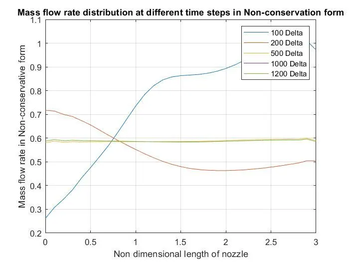
Variation of a mass flow rate distribution inside the nozzle at different time steps during the time-marching process in the Non-conservation form.

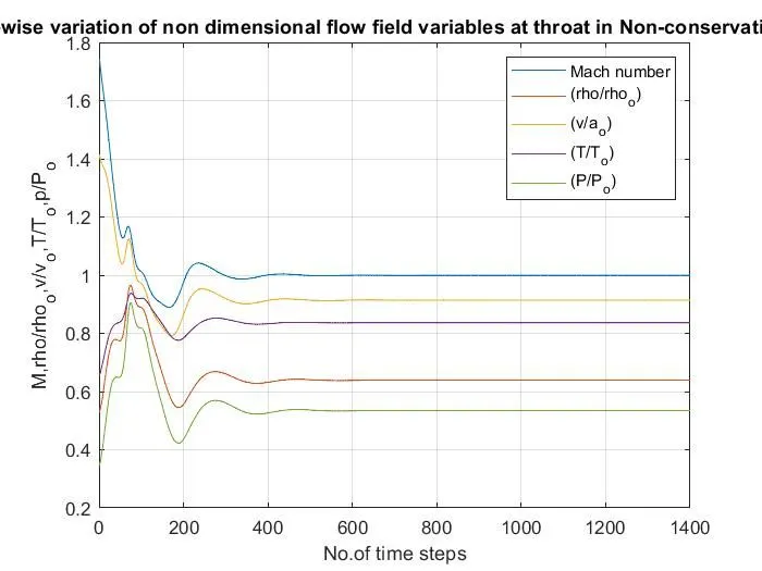
Steady-state distribution of primitive variables inside the nozzle at the throat in Non-conservation form:

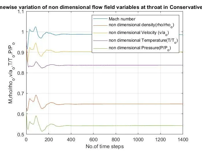
Steady-state distribution of primitive variables inside the nozzle at the throat in conservation form:

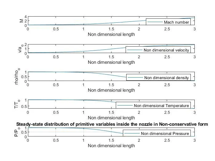
Steady-state distribution of primitive variables inside the nozzle in Non- conservation form:

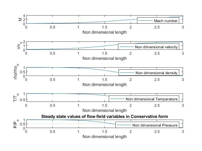
Steady-state distribution of primitive variables inside the nozzle in conservation form:

Comparison of Normalized mass flow rate distribution of Non-conservation and conservation form:

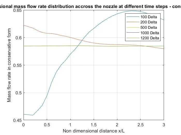
A detailed comparison of the steady-state mass flow variation was obtained with the non-conservation and conservation forms of the governing equation. The conservation form, which was much closer to the exact solution.

The comparison of the mass flow in both conservation and Non-conservation forms indicates the conservation form does a better job than the Non-conservation form as mass flow itself is a dependent variable in the equation.

Grid independence test:

The test is conducted for 31 grid points

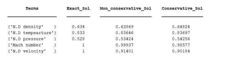
The solution is approximately matching with the results of the exact solution. Hence, the solution can be considered grid-independent.

Note that the non-conservation form results are distinctly closer to the exact values. By doubling the no. of grid points, the steady-state numerical results are slightly closer to the exact, analytical values but not as close as the non-conservation form results with half as many grid points. For all practical purposes, we have grid independence with 31 grid points.

Conclusion:

1. By observing the results of both Non-conservation and conservative forms, there is no conclusive evidence, on the best results as there is no discontinuity or shocks in the flow.
2. But for the mass flow distribution, the conservation form does a fair job because the mass flow rate is one of the dependent variables.
3. The non-conservation form produces a slightly more accurate result for the primitive variable on the other hand conservation form produces better results for flux variables. Both forms produce a satisfactory result.
4. Based on the computing effort of the solution, the conservation form takes extra effort in converting the primitive variables into flux variables for a similar result.
5. The non-conservation form attains a steady-state faster than the conservation form.