Week 3.5 - Deriving 4th order approximation of a 2nd order derivative using Taylor Table method

Objective:

To determine the difference in the error of fourth order second derivative approximations of central difference, right handed skewed difference and left handed skewed difference using Taylors table.

Introduction:

Creating Taylor tables and forming the equation for all the difference schemes.

The number of nodes in the stencil is given by

For central scheme P+Q-1 = 2+4-1=5

For skewed scheme P+Q=2+4=6

Where P is the order of the derivative

Q is the order of approximation

Taylor table for Central difference:

The fourth order second derivative central difference scheme is given by

`dx^ 2(∂ ^2u)/(∂x^2)≈a*f(i-2)+b*f(i-1)+c*f(i)+d*f(i+1)+ef(i+2)`

	f(x)	f’(x)∆x	f’’(x) ∆x2	f’’’(x) ∆x3	f’’(x) ∆x4
a*f(i-2)	a	-2a	4a/2	-8a/6	16a/24
b*f(i-1)	b	-b	b/2	-b/6	b/24
c*f(i)	c	0	0	0	0
d*f(i+1)	d	2d	4d/2	8d/6	16d/24
e*f(i+2)	e	e	e/2	e/6	e/24
Σ	0	0	1	0	0

From above table, the following equations are created

a+b+c+d+e=0

-2a-b+d+2e=0

`4a/2 +b/2 +d/2 +4e/2 =1`

`-8a/6 -b/6 + d/6 +8e/6 = 0`

`16a/24 +b/24 +d/24 + 16e/24 =0`

We have 5 equations and five variables. Use matrix method [A][X=[B] to solve the equations.

Taylor table for skewed right side difference:

The fourth order second derivative central difference scheme is given by

`dx^ 2(∂ ^2u)/(∂x^2)≈a*f(i)+b*f(i+1)+c*f(i+2)+d*f(i+3)+ef(i+4)+g(i+5)`

	f(x)	f’(x)∆x	f’’(x) ∆x2	f’’’(x) ∆x3	f’’’’(x) ∆x4	f’’’’(‘x) ∆x5
a*f(i)	a	0	0	0	0	0
b*f(i+1)	b	b	b/2	b/6	b/24	b/120
c*f(i+2)	c	2c	4c/2	8c/6	16c/24	32c/120
d*f(i+3)	d	3d	9d/2	27d/6	81d/24	243d/120
e*f(i+4)	e	4e	16e/2	64e/6	256e/24	1024e/120
g*f(i+5)	g	5g	25g/2	125g/6	625g/24	3125g/120
Σ	0	0	1	0	0	0

From above table, the following equations are created

a+b+c+d+e=0

-2a-b+d+2e=0

`4a/2 +b/2 +d/2 +4e/2 =1`

`-8a/6 -b/6 + d/6 +8e/6 = 0`

`16a/24 +b/24 +d/24 + 16e/24 =0`

We have 5 equations and five variables. Use matrix method [A][X=[B] to solve the equations.

Taylor table for skewed left side difference:

The fourth order second derivative central difference scheme is given by

`dx^ 2(∂ ^2u)/(∂x^2)≈a*f(i-5)+b*f(i-4)+c*f(i-3)+d*f(i-2)+ef(i-1)+g(i)`

	f(x)	f’(x)∆x	f’’(x) ∆x2	f’’’(x) ∆x3	f’’’’(x) ∆x4	f’’’’(‘x) ∆x5
a*f(i-5)	a	-5a	25a/2	-125a/6	625a/24	-3125a/120
b*f(i-4)	b	-4b	16b/2	-64b/6	256b/24	-1024b/120
c*f(i-3)	c	-3c	9c/2	-27c/6	81c/24	-243c/120
d*f(i-2)	d	-2d	4d/2	-8d/6	16d/24	-32d/120
e*f(i-1)	e	-e	e/2	-e/6	e/24	-e/120
g*f(i)	g	0	0	0	0	0
Σ	0	0	1	0	0	0

From above table, the following equations are created.

a+b+c+d+e+g=0

-5a - 4b -3c - 2d - e=0

`25a/2 + 16b/2 + 9c/2 + 4d/2 + e/2=1`

`-125a/6 - 64b/6 - 27c/6 - 8d/6 - e/6=0`

`625a/24 + 256b/24 + 81c/24 + 16d/24 + e/24=0`

`-3125a/120 - 1024b/120 - 243c/120 - 32d/120 - e/120=0`

We have 6 equations and 6 variables. Use matrix method [A][X=[B] to solve the equation

Solving the equations in the Matlab

close all
clear all
clc
% finding central difference coefficients
A=[1 1 1 1 1; -2 -1 0 1 2;4/2 1/2 0 1/2 4/2; -8/6 -1/6 0 1/6 8/6; 16/24 1/24 0 1/24 16/24];
B= [0;0;1;0;0];
X= inv(A)*B;
%finding skewed right side difference coefficients
C=[1 1 1 1 1 1;0 1 2 3 4 5;0 1/2 2 9/2 16/2 25/2;0 1/6 8/6 27/6 64/6 125/6;0 1/24 16/24 81/24 256/24 625/24;0 1/120 32/120 243/120 1024/120 3125/120];
D=[0;0;1;0;0;0];
Y= inv(C)*D;
%finding skewed left side difference coefficients
E=[1 1 1 1 1 1;-5 -4 -3 -2 -1 0; 25/2 16/2 9/2 2 1/2 0;-125/6 -64/6 -27/6 -8/6 -1/6 0;625/24 256/24 81/24 16/24 1/24 0; -3125/120 -1024/120 -243/120 -32/120 -1/120 0];
F=[0;0;1;0;0;0];
Z=inv(E)*F;

%Displaying the solution
%central_difference
fprintf('Central difference')
fprintf('\na=%.4f',X(1))
fprintf('\nb=%.4f',X(2))
fprintf('\nc=%.4f',X(3))
fprintf('\nd=%.4f',X(4))
fprintf('\ne=%.4f',X(5))

%skewed_right_difference
fprintf('\n\nskewed right difference')
fprintf('\na=%.4f',Y(1))
fprintf('\nb=%.4f',Y(2))
fprintf('\nc=%.4f',Y(3))
fprintf('\nd=%.4f',Y(4))
fprintf('\ne=%.4f',Y(5))
fprintf('\ng=%.4f',Y(6))

%skewed_left_difference
fprintf('\n\nskewed left difference')
fprintf('\na=%.4f',Z(1))
fprintf('\nb=%.4f',Z(2))
fprintf('\nc=%.4f',Z(3))
fprintf('\nd=%.4f',Z(4))
fprintf('\ne=%.4f',Z(5))
fprintf('\ng=%.4f',Z(6))

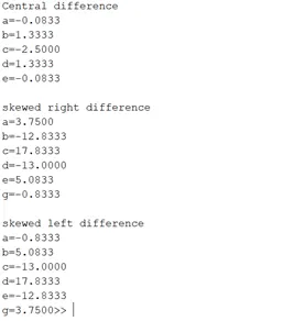
The output for the code gives you the coefficients of the terms in Taylor table

Algorithm for the code:

• Define the variable x and array dx.
• Compute the exact derivative.
• Create functions for central, right skewed, and left skewed difference which gives error of approximation for all the approximations.
• Begin for loop to create the array of error approximations over the range of dx.
• Plot the error arrays along dx.

Main code:

clc
clear all
close all

% finding central difference coefficients
A=[1 1 1 1 1; -2 -1 0 1 2;4/2 1/2 0 1/2 4/2; -8/6 -1/6 0 1/6 8/6; 16/24 1/24 0 1/24 16/24];
B= [0;0;1;0;0];
X= inv(A)*B;
%finding skewed right side difference coefficients
C=[1 1 1 1 1 1;0 1 2 3 4 5;0 1/2 2 9/2 16/2 25/2;0 1/6 8/6 27/6 64/6 125/6;0 1/24 16/24 81/24 256/24 625/24;0 1/120 32/120 243/120 1024/120 3125/120];
D=[0;0;1;0;0;0];
Y= inv(C)*D;
%finding skewed left side difference coefficients
E=[1 1 1 1 1 1;-5 -4 -3 -2 -1 0; 25/2 16/2 9/2 2 1/2 0;-125/6 -64/6 -27/6 -8/6 -1/6 0;625/24 256/24 81/24 16/24 1/24 0; -3125/120 -1024/120 -243/120 -32/120 -1/120 0];
F=[0;0;1;0;0;0];
Z=inv(E)*F;

x=pi/3;
dx=linspace(pi/4,pi/4000,20);

%function,f=exp(x)*cos(x)

%analytical  second derivative
exact_derivative=-2*exp(x)*sin(x);

for i=1:length(dx)
central_error(i)=central_difference(exact_derivative,x,dx(i),X);
skewed_right_error(i)=skewed_right_difference(exact_derivative,x,dx(i),Y);
skewed_left_error(i)=skewed_left_difference(exact_derivative,x,dx(i),Z);
end

%plotting log graph
loglog(dx,central_error,'linewidth',1,'color','r')
hold on
loglog(dx,skewed_right_error,'linewidth',1,'color','b')
loglog(dx,skewed_left_error,'linewidth',1,'color','k')
xlabel('dx(grid size)')
ylabel('error')
title('Error comparisons for numerical approximations using Taylor table method')
legend('central difference','skewed right sided difference','skewed left sided difference','location','northwest')

Central difference function:

function  error= central_difference(exact_derivative,x,dx,X)

%f(x)=exp(x)*sin(x)
%Central_difference(f''(x))=(a*f(x-2dx)+b*f(x-dx)+c*f(x)+d*f(x+dx)+e*f(x+2dx))/(dx^2)
f1= exp(x-2*dx)*cos(x-2*dx);
f2= exp(x-dx)*cos(x-dx);
f3= exp(x)*cos(x);
f4= exp(x+dx)*cos(x+dx);
f5= exp(x+2*dx)*cos(x+2*dx);
central_diff = ((X(1)*f1)+(X(2)*f2)+(X(3)*f3)+(X(4)*f4)+(X(5)*f5))/(dx^2);
error= abs(exact_derivative-central_diff);
end

The output of this function gives you the error of central difference approxiamtion.

Right skewed difference function:

function error= skewed_right_difference(exact_derivative,x,dx,Y)

%f(x)=exp(x)*sin(x)
%skewed right sided difference(f''(x))=(a*f(x)+b*f(x+dx)+c*f(x+2*dx)+d*f(x+3*dx)+e*f(x+4*dx))/(dx^2)
f1= exp(x)*cos(x);
f2= exp(x+dx)*cos(x+dx);
f3= exp(x+2*dx)*cos(x+2*dx);
f4= exp(x+3*dx)*cos(x+3*dx);
f5= exp(x+4*dx)*cos(x+4*dx);
f6= exp(x+5*dx)*cos(x+5*dx);
skewedright_diff= ((Y(1)*f1)+(Y(2)*f2)+(Y(3)*f3)+(Y(4)*f4)+(Y(5)*f5)+(Y(6)*f6))/(dx^2);
error= abs(exact_derivative-skewedright_diff);
end

The output of this function gives you the error of the right skewed difference approximation.

Left skewed difference function:

function error= skewed_left_difference(exact_derivative,x,dx,Z)

%f(x)=exp(x)*sin(x)
%skewed left sided difference=(a*f(x-4*dx)+b*f(x-3*dx)+c*f(x-2*dx)+d*f(x-dx)+e*f(x))/(dx^2)
f1= exp(x-5*dx)*cos(x-5*dx);
f2= exp(x-4*dx)*cos(x-4*dx);
f3= exp(x-3*dx)*cos(x-3*dx);
f4= exp(x-2*dx)*cos(x-2*dx);
f5= exp(x-dx)*cos(x-dx);
f6= exp(x)*cos(x);
skewedleft_diff= ((Z(1)*f1)+(Z(2)*f2)+(Z(3)*f3)+(Z(4)*f4)+(Z(5)*f5)+(Z(6)*f6))/(dx^2);
error= abs(exact_derivative-skewedleft_diff);
end

The output of this function gives you the error of the left skewed difference approximation.

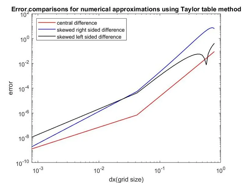
Results and plot:

Conclusion:

• The central difference approximation has less error for a given dx compared to the left and right approximation.
• The left and right sided approximation have fairly same error.
• The limitation for the central difference is that it cant be applied for a boundary as it requires points from both ends.
• Unlike central difference, the left and right sided approximation has no limitations for boundary domains.

.