Week 1- Mixing Tee

Aim:

• Set up steady-state simulations to compare the mixing effectiveness when the hot inlet temperature is 36C, and the cold inlet is 19C.
• Try both the k-epsilon and k-omega SST models for the first case to get proper judgment about each method; later, use the most suitable model for further simulations.
• Simulate each case for the given velocity and momentum ratio.
• Compare results from the 2 cases about cell count, average outlet temperature, and the number of iterations for convergence.
• Plot the velocity and temperature contour plots on the cut plane along and across the pipe.
• Also, plot the velocity and temperature line plots along and across the length of the pipe.
• Perform Mesh independent study for any one case.
• Moreover, discuss the effect of length and momentum ratio on results.

Problem Setup

Understand k-epsilon and k-omega SST by considering case-1 also grid independency done on case 1

Case-1

Short mixing tee

a - Simulation-1

hot Inlet velocity - 3m/s

Momentum ratio - 2

b - Simulation-2

hot Inlet velocity - 3m/s

Momentum ratio - 4

Case-2

Long mixing tee

a - Simulation-3

hot Inlet velocity - 3m/s

Momentum ratio - 2

b - Simulation-4

hot Inlet velocity - 3m/s

Momentum ratio - 4

procedure:

• Understand and define the problem statement for each case.
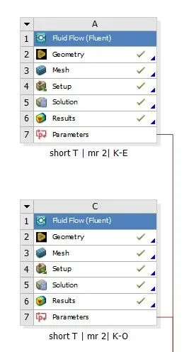
• Open Ansys workbench and set up a fluent simulation setup, and rename it accordingly.
• From fluent setup, open space claims, and Load the geometry. Extract the working fluid region from the loaded geometry to compute simulation in that particular region. And then close space claim.
• Next, in the mesh setup, provide boundary names for each surface and generate mesh to the fluid flow volume. Close mesh setup and update the mesh.
• Later, in the setup section, provide all the required parameters according to the simulation, such as simulation type, input velocity and temperature, materials (working fluid), and other user-defined parameters.
• In setup parameters, understand the concept of k-epsilon and k-omega SST and find out which is convenient for the current simulation.
• Afterward, simulate our problem setup for the number of iterations required to converge our results.
• Then, close and update the setup. Open the results section to see all the simulated results.
• Juxtapose generated results from each case for their cell count, average outlet temperature, and the number of iterations for convergence.
• Display contour plot on the cut plane to visualize velocity and temperature distribution along and across the mixing tee’s length.
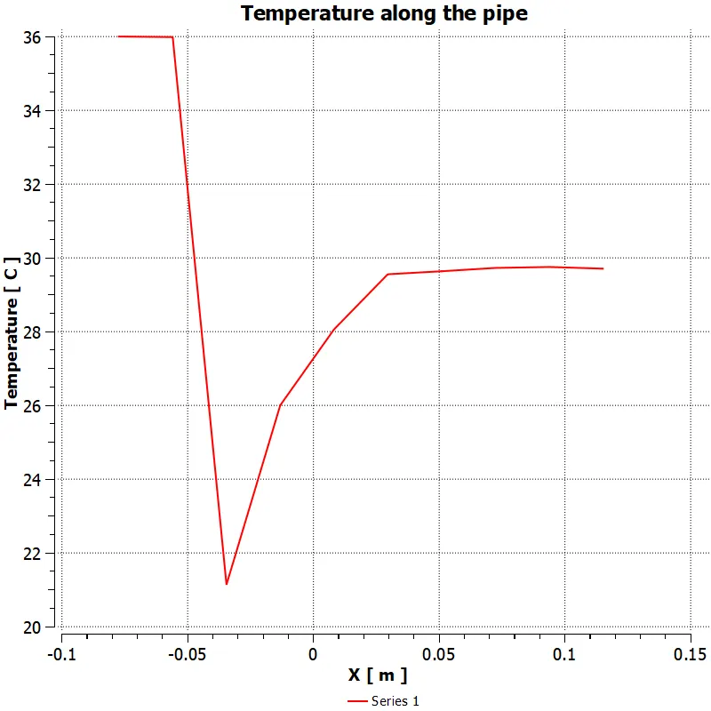
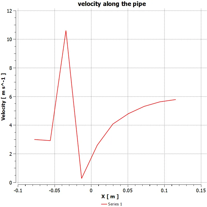
• For a more detailed examination, plot velocity and temperature line chart along the mixing tee’s length.
• Validate the test by performing a mesh independence study on any one case.
• Study the effect of length and momentum ratio on the results of each case.
• Plot the convergence graph to verify that all the results are fully converged after running numerous iterations.

Let us start with analyzing the best method to converge the solution for this particular case by studying two methods: k-epsilon and k-omega SST.

The aforementioned methods use simulation of turbulence modeling where k-epsilon models predict flow virtually far from the boundaries (wall), and the k-omega model predicts near the wall.

The selection of the model depends on the specific problem; no turbulence model suit for every case. Fine-tuning requires the SST model that used good mesh at the boundary, and with wall treated usually works in most cases; it is problem specific.

Our first study will set two setups, one for k-epsilon realizable and another for k-omega SST. Here, we are going to use the same geometry and mesh for both cases of simulation. Hence, we are going to use a short mixing tee model and mesh it.

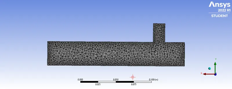
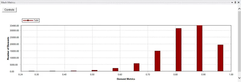
we can check the interior nodes of the mesh by sectioning the geometry. we can also improve the quality of the mesh by looking at the element metrics. the same mesh was used for both the k- epsilon realizable and k-omega SST.

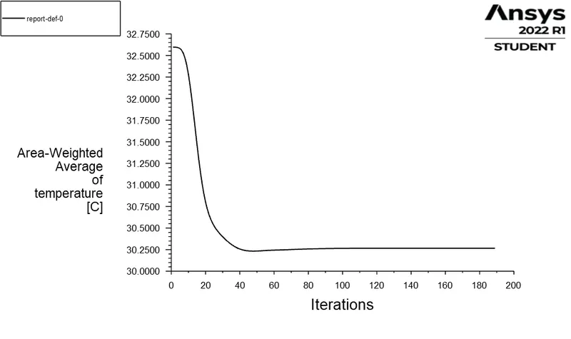
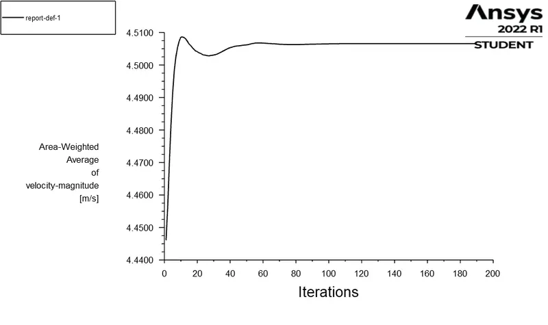
The convergence plots for the K-Epsilon model:

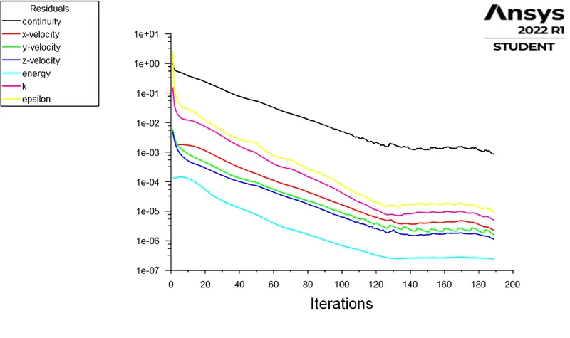
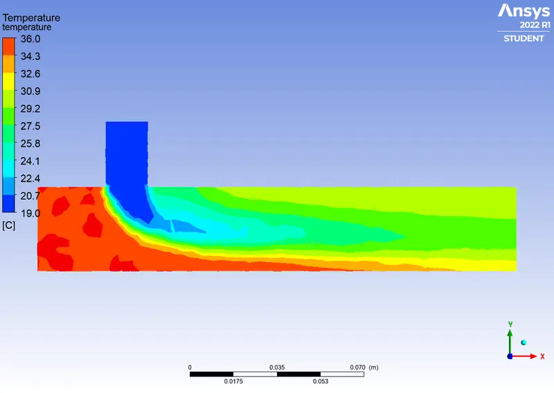
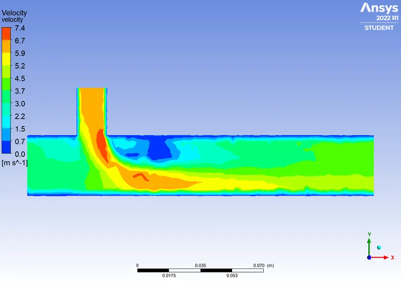
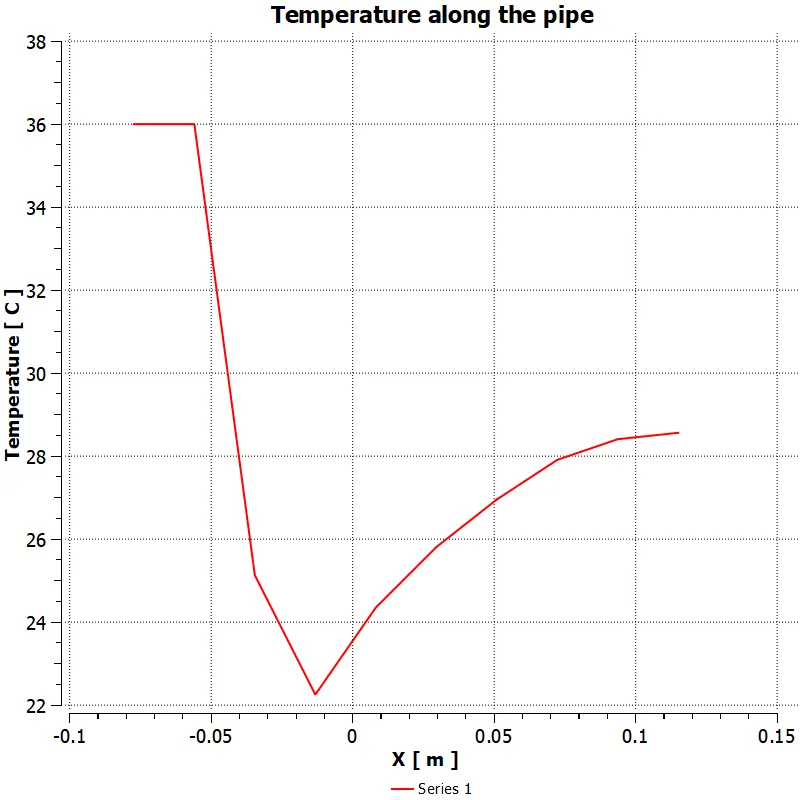
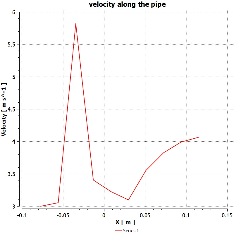
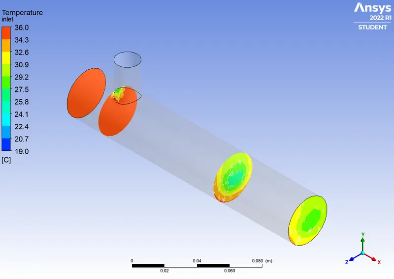
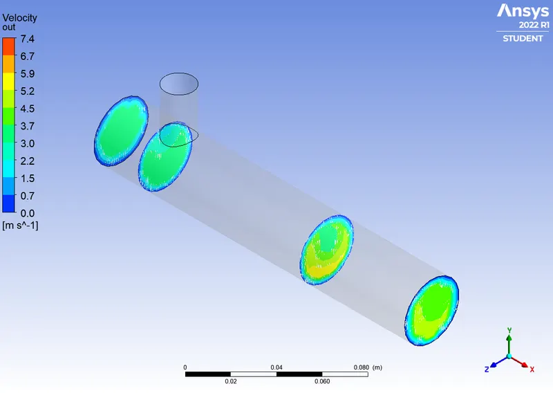
Results of K-epsilon model:

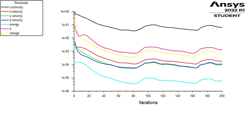
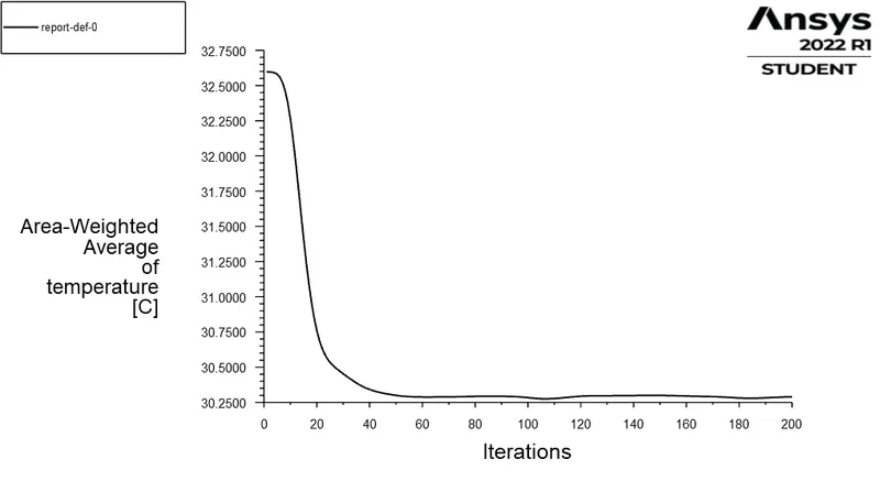
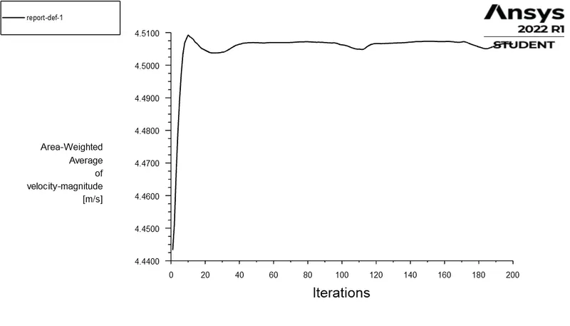
The convergence of K-Omega model:

Results of K-Omega plot:

Inference:

k-Epsilon

In the first simulation, the K-epsilon turbulence model is the most common model used in CFD to simulate mean flow characteristics for turbulent flow conditions. It is a two-equation model that gives a description of turbulence by means of two transport equations (PDEs). the first transported variables are the turbulent kinetic energy (k) and the second transported variable is the rate of dissipation of turbulent kinetic energy.

k-epsilon focuses on the mechanism that affects the turbulent kinetic energy.

k-omega SST

The SST k-omega turbulence model is a two-equation eddy-viscosity model that is used for many aerodynamic applications. It is a hybrid model combining the Wilcox k-omega and the k-epsilon models. A blending function activates the Wilcox model near the wall and the k-epsilon model in the free stream. This ensures that the appropriate model is in the free stream. This ensures that the appropriate model is utilized through the flow field.

Main difference

The k- omega model is well suited for simulating flow in the viscous sub-layer. On the contrary, The k-epsilon model is ideal for predicting flow in the regions away from the wall

The SST model exhibit less sensitivity to free stream conditions (Flow outside the boundary layer) than many other turbulence models.

The shear stress limiter helps the k-omega model avoid a build-up of excessive turbulent kinetic energy near stagnation points.

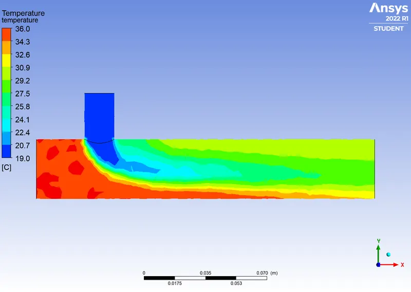
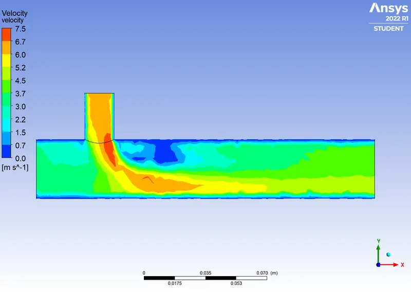
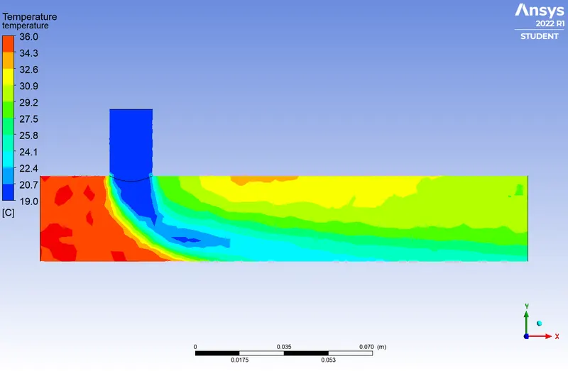
If we observe our simulated figure, we can notice, in the k-omega model flow is more like laminar and does not give proper turbulent results, in contrast, simulation by k-epsilon, is giving proper mixing of the two air streams.

In this particular case we are not dealing with walls, therefore, we are going to use the k-epsilon method for further simulations.

case 1a is already performed in the aforementioned case as K-Epsilon realizable.

the grid independency was performed for the first case for the element size of 0.005m and 0.002m.

however, the convergence and contour plots of those cases will not be shown considering the length of the report but can be tabulated to prove the grid independence.

now, we look at the simulation of case 1b:

the converge plots

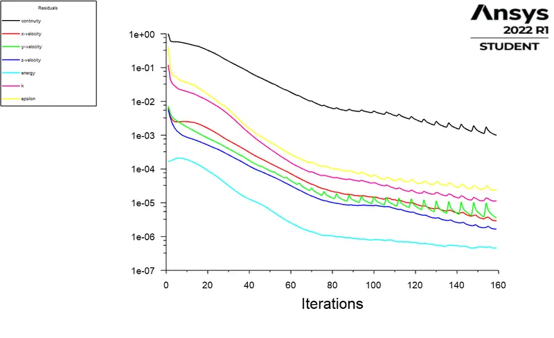
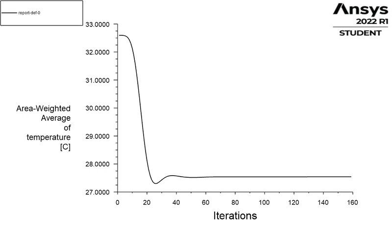
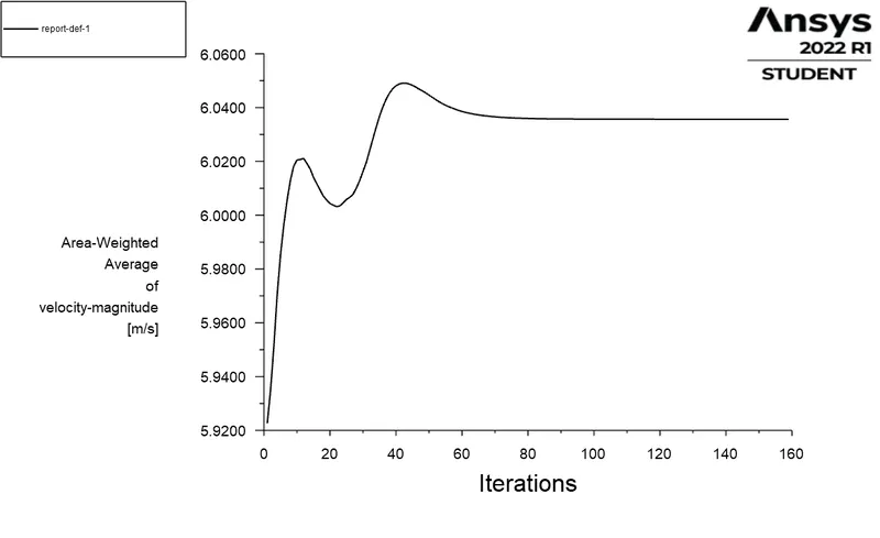
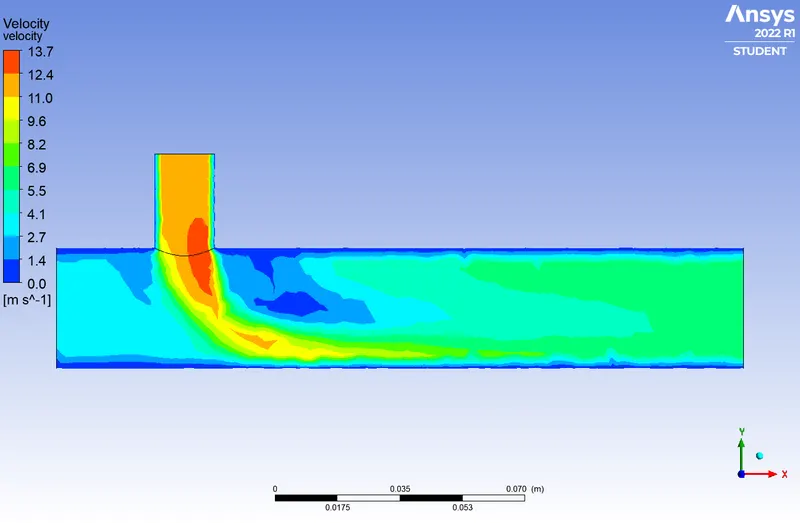
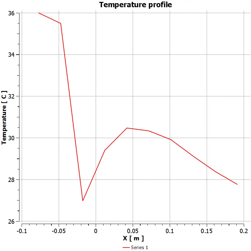
contour and line plots of case 1b:

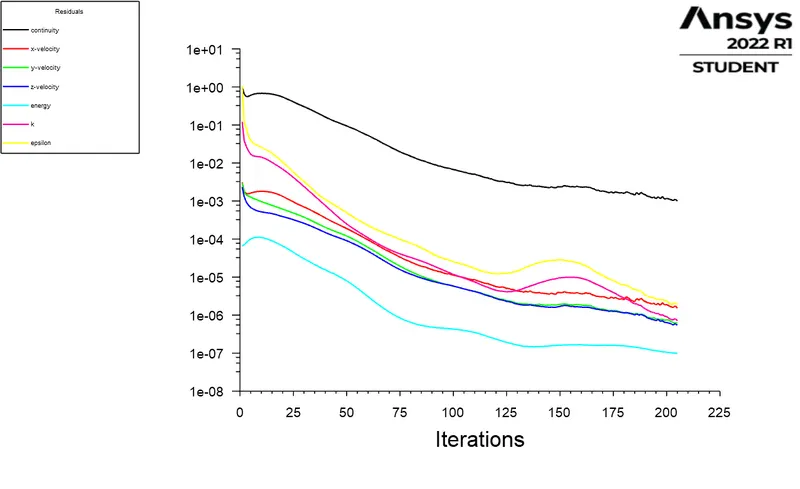
Convergence plot of case 2a :

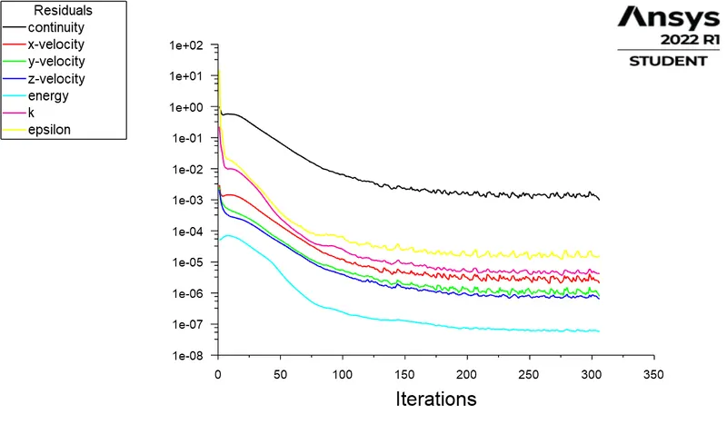
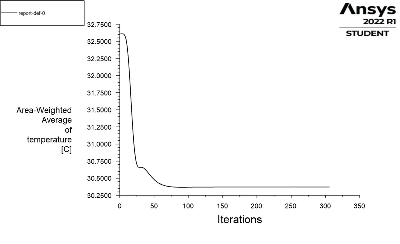
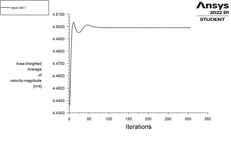
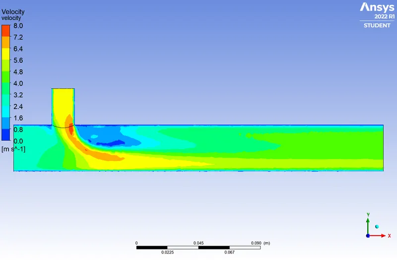
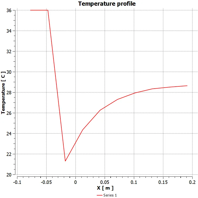
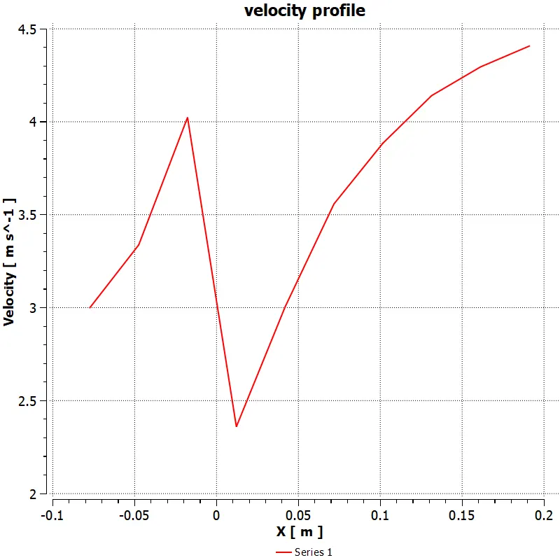
contour and line plots of case 2a:

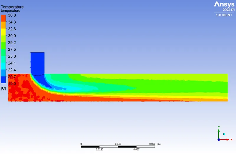
Convergence plot of case 2b:

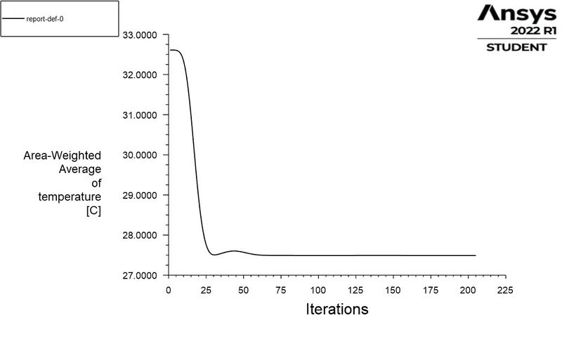
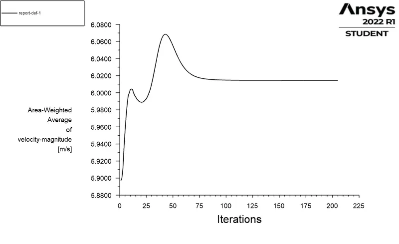
contour and line plots of case 2b:

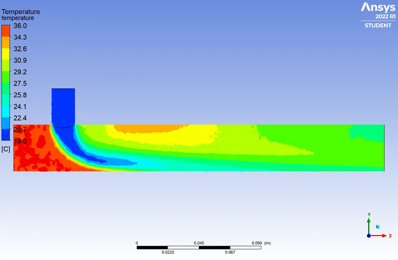
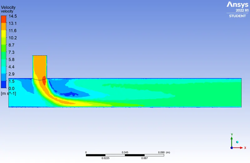
Effectiveness of mixing:

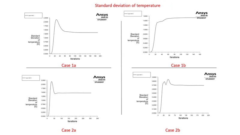
In order to measure the effectiveness of the mixing, we can calculate the standard deviation of the temperature at the outlet of the mixing tee.

A high standard deviation means the mixing is bad, on the contrary, a low standard deviation means we are getting better mixing.

Below, the line chart exhibits the standard deviation of the temperature at the outlet of the mixing tee for each case we have studied.

Now we can see in both short and long pipe the standard deviation is constantly lower after 80^th iterations which have a higher velocity of 12m/s at the cold air inlet.

Therefore, we are getting the best mixing when the flow is high and the effectiveness of mixing is almost less dependent on the length of the mixing tee

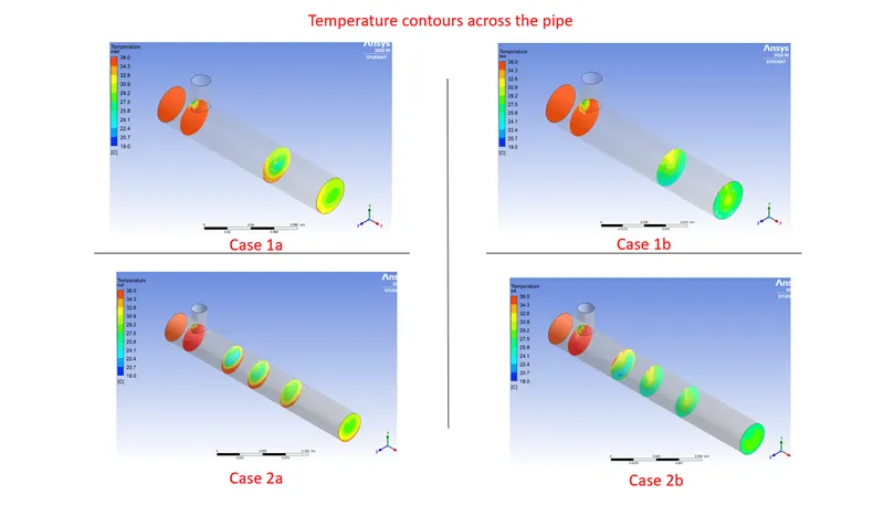
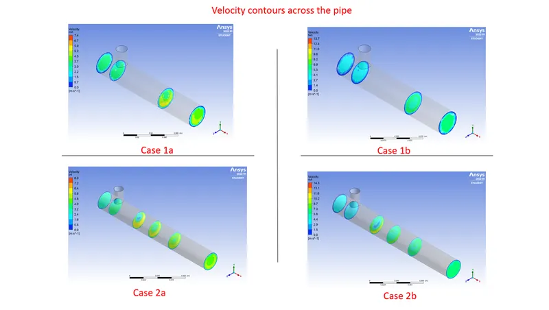
In the above figures, we took planes across the length of the mixing tee, from the middle part to the outlet of the flow.

Glimpse over the contour over plane depicts the same results of the effectiveness of mixing in is better when the flow of the fluid is higher.

the same phenomenon applies to velocity as well.

Grid independency results:

Short pipe
Momentum ratio -2
Element size	Cell count	Average outlet temperature	Average outlet velocity	number of iterations
0.005	14400	30.25	4.53	187
0.002	106587	30.3	4.56	157
Short pipe
Momentum ratio -4
Element size	Cell count	Average outlet temperature	Average outlet velocity	number of iterations
0.005	14400	27.6	6.025	159
0.002	106587	27.6	6.025	206
Long pipe
Momentum ratio -2
Element size	Cell count	Average outlet temperature	Average outlet velocity	number of iterations
0.002	140990	30.03	4.56	306
Long pipe
Momentum ratio -4
Element size	Cell count	Average outlet temperature	Average outlet velocity	number of iterations
0.002	140990	27.6	6.02	205

After putting all the results in a single table we can compare our results where we can see the length of the mixing tee does not affect the results at the output that much if we ignore the diffusion criteria.

High-velocity flow shows good mixing results than low-velocity flow.

The results passed the mesh independence criteria.

conclusion:

• k-epsilon models predict flow virtually far from the boundaries (wall), and the k-omega model predicts near the wall.
• As in this case we need a flow simulation turbulent model far from the wall, therefore, the k-epsilon method is used.
• To get better mixing at the outlet high velocity of flow is very effective. Therefore, a higher momentum ratio gives better mixing of hot and cold fluid streams at the outlet.
• As the Length of the mixing tee increases because diffusion flow always gives slightly better mixing of two-fluid.
• Finally, in the above cases, it is very important to use a short mixing tee with a momentum ratio of 4 to get precise results but one has to consider the diffusion of flow along the length of the mixing tee, a long mixing tee with momentum will be the greater option.