Week 5.1 - Mid term project - Solving the steady and unsteady 2D heat conduction problem

Objective:

To solve 2D steady state equation using steady and unsteady state analysis using

point iterative technique

1.Jacobi

2. Gauss seidel
3. Successive over-relaxation

For transient heat equation, solve both explicit and implicit equation. Plot the temperature distribution for all the cases.

Theory:

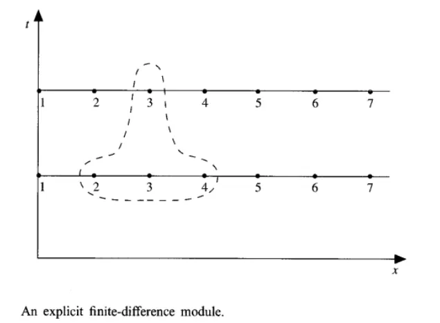
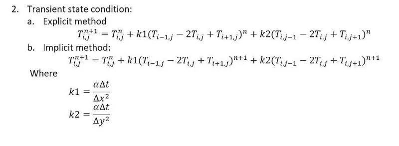
Explicit method:

In an explicit approach, each difference equation contains only 1 unknown and be therefore solved directly from the known values.

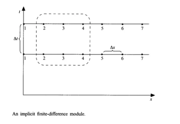
Implicit method:

The unknown values at (n+1) time step is expressed both in n and (n+1) time steps

Iterative methods:

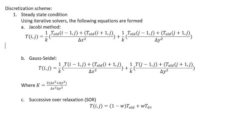
An iterative method is a mathematical procedure that uses an initial guess to generate a sequence of improving approximations solutions for a class of problems, in which the nth approximation is derived from the previous ones.

1. Jacobi method:

Jacobi method is an iterative method where all updated values are used for the computations only after all the variables have been updated.

2. Gauss-Seidel method:

Gauss-Seidel method is an iterative method, where the updated variables are used in the computations as soon as they are updated.

3. Successive over-Relaxation (SOR):

SOR is a variant of the Gauss-Seidel method for solving a system of linear equations, resulting in faster convergence. It is also used for slowly converging iterative processes. If relaxation factor <1 then the method is under-relaxed. relaxation factor >1 then the method is over-relaxed.

Governing equation:

1. 2D steady state heat conduction equation is given by

`\frac{\partial^2T}{\partial x^2}+\frac{\partial^2T}{\partial y^2}=0`

2.2D transient state heat conduction equation is given by

`\frac{\partial T}{\partial t}+\alpha(\frac{\partial^2T}{\partial x^2}+\frac{\partial^2T}{partial y^2})=0`

Boundary Condition:

Here the boundary condition is given as

T_left = 400K

T_right=800K

T_top=600K

T_bottom=900K

Initial condition is assumed to be 300K for faster convergence.

steady-state code algorithm:

Get the input values, create the grid and define the boundary condition

Calculate the corner points and assume the interior nodes to be 300 K for faster convergence.

Define constant K , error and tolerance.

Define old t values and initialize the iterations.

Ask user for the iteration method

Based on the iteration method, start the solution with checking whether the error is more than the tolerance and continue the iteration

Start the space loop and calculate the temperatures using the following equation

term1=(told1(i-1,j)+told1(i+1,j))/(dx^2);

term2=(told1(i,j-1)+told1(i,j+1))/(dy^2);

t(i,j)=(term1+term2)/k;

Update the old t values and increment the iteration count

Before checking the error for next iteration calculate error.

Now, plot the temperature distribution of the solution using contour plot.

Repeat the same procedure for the rest of the iterative solvers with slight change in the equation which are represented below.

Steady state code:

clc
clear all
close all

% inputs
L=1;
nx=10;
ny=10;
x=linspace(0,L,nx);
y=linspace(0,L,ny);
dx=x(2)-x(1);
dy=y(2)-y(1);

% boundary conditions
t_left = 400;
t_top = 600;
t_right = 800;
t_bottom = 900;
t = ones(nx,ny);
% Temperature at boundary
t(2:nx - 1,1) = t_left;
t(2:nx - 1,ny) = t_right;
t(1,2:ny - 1) = t_top;
t(nx,2:ny - 1) = t_bottom;

% corner points
t(1,1) = (t_top + t_left)/2;
t(nx,ny) = (t_right + t_bottom)/2;
t(1,ny) = (t_top + t_right)/2;
t(nx,1) = (t_left + t_bottom)/2;

% assumption
t(2:nx-1,2:ny-1)= 300;

%  creating the meshgrid
[xx yy]=meshgrid(x,y);
k=(2*(dx^2+dy^2)/((dx^2)*(dy^2)));

% assume error to start the iterations
error=9e9;
tol=1e-4;

% create the t old variable for all the schemes
told1=t;
told2=t;
told3=t;
method=0;

% initializing the iteration
tinitial=t;
j_iter=1;
gs_iter=1;
sor_iter=1;
w=0;
method=input('Enter method number 1.Jacobi 2.Gauss Seidel 3.SOR\n')

%Jacobi
if(method==1)
    while error>tol
        for i=2:nx-1
            for j=2:ny-1
                term1=(told1(i-1,j)+told1(i+1,j))/(dx^2);
                term2=(told1(i,j-1)+told1(i,j+1))/(dy^2);
                t(i,j)=(term1+term2)/k;
                
            end
        end
        
        %find the error between old and new t values
        error=max(max(abs((t-told1))));
        
        %update old t values
        told1=t;
        
        %update the iteration count
        j_iter=j_iter+1;
    end
    
    contourf(x,y,t,'showtext','on')
    colormap(jet)
    colorbar
    set(gca,'YDIR','reverse')
    
    xlabel('X axis')
    ylabel('Y axis')
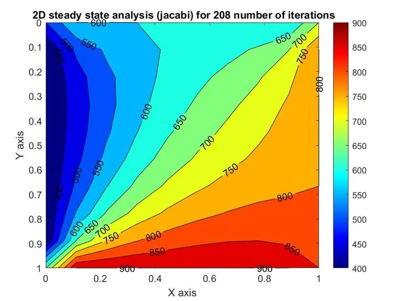
    title(sprintf(' 2D steady state analysis (jacabi) for %d number of iterations',j_iter))
    pause(0.02)   
            
end

%Gauss Seidel
if(method==2)
while error>tol
for i=2:nx-1
for j=2:ny-1
term1= (t(i-1,j)+told2(i+1,j))/(dx^2);
term2= (t(i,j-1)+told2(i,j+1))/(dy^2);
 
        t(i,j)=(term1+term2)/k ;
end
end
error=max(max(abs(t-told2)));
told2=t;
gs_iter=gs_iter+1;
end
contourf(x,y,t,'showtext','on')
colormap(jet)
colorbar
set(gca,'YDIR','reverse')
xlabel('X axis')
ylabel('Y axis')
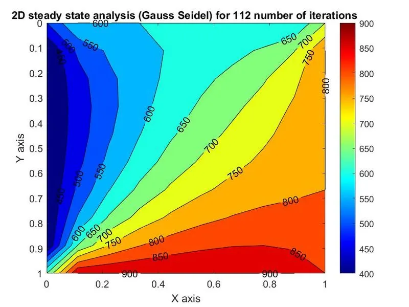
title(sprintf('2D steady state analysis (Gauss Seidel) for %d number of iterations ',gs_iter))
pause(0.02)
end

% Successive Over-relaxation
if(method==3)
w=input('Enter omega value >1 for succesive over relaxation')
while error>tol
for i=2:nx-1
for j=2:ny-1
term1= (t(i-1,j)+told3(i+1,j))/(dx^2);
term2= (t(i,j-1)+told3(i,j+1))/(dy^2);
t(i,j)=(term1+term2)/k ;
t(i,j)=(1-w)*told3(i,j) + w.*t(i,j) ;
end
end
error=max(max(abs((t-told3))));
told3=t;
sor_iter=sor_iter+1;
end
contourf(x,y,t,'showtext','on')
colormap(jet)
colorbar
set(gca,'YDIR','reverse')
xlabel('X axis')
ylabel('Y axis')
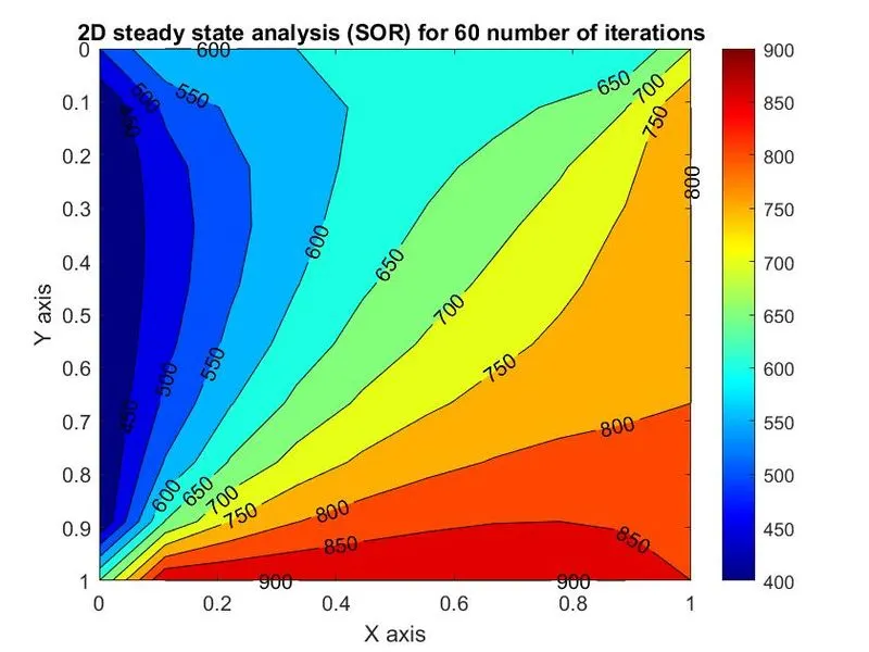
title(sprintf('2D steady state analysis (SOR) for %d number of iterations ',sor_iter))
pause(0.02)
end

Output:

Transient state code algorithm:

Get the input values and create grid and boundary conditions.

Calculate the outer and corner points and update the grid.

Assume the interior points to be at 300 for faster convergence.

Assign the error and old t values

Initialize the iterations and assume the diffusivity and time steps.

Since, it is transient state we have both implicit and explicit methods.

Consider the CFL number to be less than 0.25 for Explicit and any value for the Implicit as it is unconditionally stale.

Like the study state use space loop and additional time loop for the solution

Find the error and compare with the tolerance and start the next iteration

Update the t_old values before starting next time step.

Plot the contour plot of the grid

Transient state code:

clc
clear all
close all

% inputs
L=1;
nx=10;
ny=10;

% setting up the grid
x=linspace(0,L,nx);
y=linspace(0,L,ny);
dx=x(2)-x(1);
dy=y(2)-y(1);
[xx,yy]=meshgrid(x,y);

% boundary conditions
t_left = 400;
t_top = 600;
t_right = 800;
t_bottom = 900;
t = ones(nx,ny);

% Temperatures at boundary
t(2:nx - 1,1) = t_left;
t(2:nx - 1,ny) = t_right;
t(1,2:ny - 1) = t_top;
t(nx,2:ny - 1) = t_bottom;

% corner points
t(1,1) = (t_top + t_left)/2;
t(nx,ny) = (t_right + t_bottom)/2;
t(1,ny) = (t_top + t_right)/2;
t(nx,1) = (t_left + t_bottom)/2;

% assumption
t(2:nx-1,2:ny-1)= 300;

% value of k
% k=(2*(dx^2+dy^2)/((dx^2)*(dy^2)));

% assigning the old values
error=9e9;
tp=t;
tol=1e-4;
told1=t;
told2=t;
told3=t;
% method=0;

% initializing iterations
told=t;
counter=1;
j_iter=1;
gs_iter=1;
sor_iter=1;
w=0;
    
a1=1e-2;
dt=30;
nt=2000;
k=a1*dt/(dx^2);
%CFL number to check for stability condition
CFL=a1*dt/(dx^2);

method=input('enter method 1.explicit 2.implicit jacobi 3.implicit Gauss seidel 4. implicit SOR \n');
if(method==1)
tic
 a1=0.02;
 t_tot=10;
 dt=0.1;
 nt=t_tot/dt;

% k1=a1*dt/(dx^2),k2=a1*dt/(dy^2)
% since it's a symmetric grid k1=k2=k. it applies for both implicit and
% explicit schemes

k=a1*dt/(dx^2);
CFL=a1*dt/(dx^2);

% Explicit scheme

% time loop
tic;
for h=1:nt
%     space loop
for i=2:nx-1
for j=2:ny-1
term1= (told(i-1,j)-(2*told(i,j))+told(i+1,j));
term2= (told(i,j-1)-(2*told(i,j))+told(i,j+1));
t(i,j)=told(i,j)+k*(term1+term2) ;

end
end
error =max(max(abs(told-t)));
counter=counter+1;
told=t;
end
time= toc;
% To plot contour (same code for all cases)
contourf(x,y,t,'showtext','on')
colormap(jet)
colorbar
set(gca,'YDIR','reverse')
xlabel('X axis')
ylabel('Y axis')
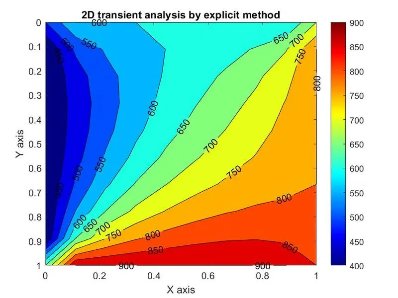
title(sprintf('2D transient analysis by explicit method'))
pause(0.02)
sprintf('The Time required for the solution is %f',time)
sprintf('The number of iterations are %f',counter)
end

%Implicit scheme
if (method==2)
    tic
% Time loop
for h=1:nt
while error>tol
% Space loop
for i=2:nx-1
for j=2:ny-1
    
term1=(1+(4*k))^-1;
term2=k*term1;
H=(told(i-1,j)+told(i+1,j));
V=(told(i,j-1)+told(i,j+1));
t(i,j)=(tp(i,j)*term1)+(H*term2)+(V*term2);

end
end
 error=max(max(abs((t-told))));
told=t;
j_iter=j_iter+1;
end
tp=told;
end
time= toc
contourf(x,y,t,'showtext','on')
colormap(jet)
colorbar
set(gca,'YDIR','reverse')
xlabel('X axis')
ylabel('Y axis')
title(sprintf('2D transient analysis by implicit Jacobi method'))
pause(0.02)
sprintf('The Time required for the solution is %f',time)
sprintf('The number of iterations are %f',j_iter)
end

% Gauss Seidel
if (method==3)
    tic
for h=1:nt
while error>tol
for i=2:nx-1
for j=2:ny-1
term1=(1+(4*k))^-1;
term2=k*term1;
H=(t(i-1,j)+told2(i+1,j));
V=(t(i,j-1)+told2(i,j+1));
t(i,j)=(tp(i,j)*term1)+(H*term2)+(V*term2);
end
end
error=max(max(abs((t-told2))));
told2=t;
gs_iter=gs_iter+1;
end
tp=told;
end
time= toc
contourf(x,y,t,'showtext','on')
colormap(jet)
colorbar
set(gca,'YDIR','reverse')
xlabel('X axis')
ylabel('Y axis')
title(sprintf('2D transient analysis by implicit Gauss Seidel method'))
pause(0.02)
sprintf('The Time required for the solution is %f',time)
sprintf('The number of iterations are %f',gs_iter)
end

%SOR
if (method==4)
    tic
w=input('Enter omega value for succesive over relaxation')
% time loop
for h=1:nt
%     space loop
while error>tol
for i=2:nx-1
for j=2:ny-1
term1=(1+(4*k))^-1;
term2=k*term1;
H=(t(i-1,j)+told3(i+1,j));
V=(t(i,j-1)+told3(i,j+1));
t(i,j)=(tp(i,j)*term1)+(H*term2)+(V*term2);
t(i,j)=(1-w)*told3(i,j) + w.*t(i,j);
end
end
error=max(max(abs((t-told3))));
told3=t;
sor_iter=sor_iter+1;
end
tp=told;
end
time= toc
contourf(x,y,t,'showtext','on')
colormap(jet)
colorbar
set(gca,'YDIR','reverse')
xlabel('X axis')
ylabel('Y axis')
title(sprintf('2D transient analysis by implicit SOR method'))
pause(0.02)
sprintf('The Time required for the solution is %f',time)
sprintf('The number of iterations are %f',sor_iter)
end

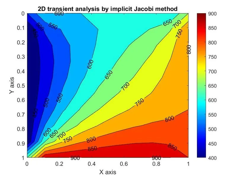
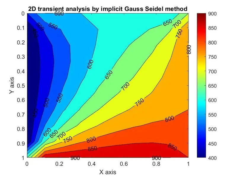
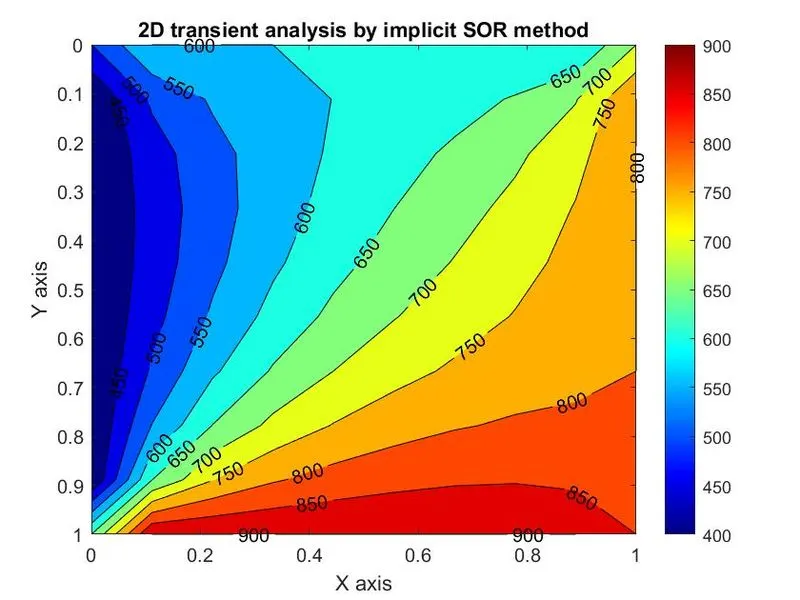
Output:

Conclusion:

The computational time and iteration required are SOR<GS<JACOBI for both steady and unsteady states. The implicit method can be used to problems when converged results are needed in less computation time as they are unconditionally stable. With increases in time step size, the convergence rate is increased which leads to a steady-state with less no. of iterations. The explicit method results in time-accurate solutions as it is governed by stability criteria when not satisfied it leads to an unstable solution and requires more iterations to attain a steady-state. Explicit approach information from a given cell or mesh element must propagate to its immediate neighbors, hence the low CFL number needs to be considered.

Hence for this time step size, the explicit scheme leads to a faster convergent rate and as the time step size is small the number of iterations increases for the implicit scheme which results in slower convergence rate.