Week 7 - Simulation of a 1D Super-sonic nozzle flow simulation using Macormack Method
Note: CFD book by John Anderson is refered for Initial and boundary conditions.
AIM:- To simulate the isentropic flow through a quasi 1D subsonic-supersonic nozzle for Conservative and Non-Conservative forms of the governing equations.
Objective:-
- Using MacCormack's technique simulate the isentropic flow through a quasi 1D subsonic-supersonic nozzle for Conservative and Non-Conservative forms of the governing equations
- Determine the steady-state temperature distribution for the flow-field variable
- You need to show the following plots inside your report
1. Steady-state distribution of primitive variables inside the nozzle
2. Time-wise variation of the primitive variables
3. Variation of Mass flow rate distribution inside the nozzle at different time steps during the time-marching process
4. Comparison of Normalized mass flow rate distributions of both forms
Theory:-
NOZZLES- A nozzle (from the nose, meaning 'small spout') is a tube of varying cross-sectional area (usually axisymmetric) aiming at increasing the speed of an outflow, and controlling its direction and shape. Nozzle flow always generates forces associated with the change in flow momentum, as we can feel by handholding a hose and opening the tap.
In the simplest case of a rocket nozzle, relative motion is created by ejecting mass from a chamber backward through the nozzle, with the reaction forces acting mainly on the opposite chamber wall, with a small contribution from nozzle walls.
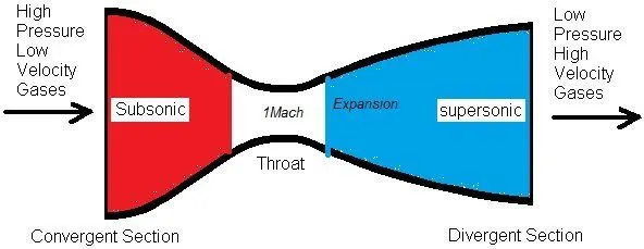
A converging-diverging nozzle ('condi' nozzle, or CD-nozzle), is the only one to get supersonic flows with M>1 (when chocked)
Assumptions:-
- We consider the steady, isentropic flow through a convergent-divergent nozzle as sketched in Fig 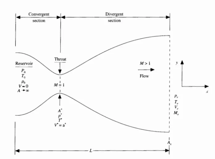
- The flow at the inlet to the nozzle comes from a reservoir where the pressure and temperature are denoted by `P_0`, and `T_0`, `P_0` and `T_0` are the stagnation values, or total pressure and total temperature, respectively.
- The cross-sectional area of the reservoir is large ( theoretically, A `rightarrow infty` ), Hence the velocity is very small ( V `rightarrow 0` )
- The flow expands isentrop1cally to supersonic speeds at the nozzle exit, where the exit pressure, temperature, velocity, and Mach number are denoted by `P_e,T_e,V_e and M_e` respectively.
- The flow is locally subsonic in the convergent section of the nozzle, sonic at the throat(minimum area), and supersonic at the divergent section.
- The Sonic flow(M = 1) at the throat means that the local velocity at this location is equal to the local speed of sound.
- Sonic flow values, we have at the throat V = V* = a*, and the sonic flow values of pressure and temperature are denoted by p* and T*, respectively. The area of the sonic throat is denoted by A*
- We assume that at a given section, where the cross-sectional area is A, the flow properties are uniform across that section. Hence, although the area of the nozzle changes as a function of distance along with the nozzle, x, and therefore in reality the flow field is two-dimensional (the flow varies in the two-dimensional .xy space), we make the assumption that the flow properties-vary only with x; this is tantamount to assuming uniform flow properties across any given cross-section. Such flow is defined as quasi-one-dimensional flow.
Quasi 1D flow-
- In quasi-1-D flow, cross-section varies as a Function of the longitudinal coordinate, x.
- Flow Properties are assumed constant across any cross-section.
- x-axis is the direction of flow, there is no flow along the y-axis, z-axis.
NOTE:- It is Quasi 1D flow, as we are assuming it is 1D flow, but in reality, it is actually a minimum of 2D.
Governing Equation:-
The governing continuity, momentum, and energy equations for this quasi-one-dimensional, steady, isentropic flow can be expressed, respectively, as
Continuity- `rho_1 V_1 A_1 = rho_2 V_2 A_2`
Momentum- `rho_1 A_1 + rho_1 V_1^2 A_1 + int_(A_1)^(A_2) rho dA = rho_2 A_2 + rho_2 V_2^2 A_2`
Energy- `h_1 + V_1^2/2 = h_2 + V_2^2/2`
Conservation and Non-conservation:-
- The conservative and non-conservative forms of the Navier-Stokes equations are mathematically the same. The difference comes when discretizing the equations. Notice that both the non-conservative and conservative forms come from the conservation equations (i.e. conservation of mass and conservation of momentum). So, you can have both a conservative form of the conservation equations and a non-conservative form of the conservation equations.
Non-conservative form: `(Dp)/(Dt) + rho nabla V =0`
Conservative form: `(del rho)/(del t) + nabla(rho V) = 0`
- In the conservation form, the derivation is made under the assumption that the control volume is fixed and hence the variation of density with respect to time is provided by the local derivative while in the case of the non-conservation form, the derivation is made under the assumption that the control volume is moving.
- Here, the variation of density with respect to time is given by the sum of the local derivative(variation due to unsteady nature) and the convective derivative(variation due to moving control volume)
- The conservative form derives from expressing the conservation equations in a divergence form, i.e. the equations have the form of the local time rate of change + divergence of flux = source terms. A non-conservative form is a form of the equations that are not expressible in this form. One of the principal advantages to the conservative form is that once the equations are discretized, the flux terms "telescope", that is if you sum the fluxes into and out of a row of cells, the intercell fluxes cancel and the net flux is just the flux out of one end of the row - flux in the other end.
- Conservative form has an advantage: its integral form allows discontinuous solutions (leading to Rankine-Hugoniot relation and correct shock speed). The non-conservative form does not have such a character (it allows only smooth differentiable solutions).
MacCormack's technique:-
- The Maccormack method is also an explicit finite-difference technique that is second-order-accurate in both space and time. The results obtained by using MacCormack's method is perfectly satisfactory for many fluid flow applications
- First, we start with the initial condition and then calculate the value for the next time step, but this is not the entire time step, it is basically the Predator step.
Predator step- We assume that the flow field at each grid point is known at time t, and we proceed to calculate the flow-field variables at the same grid points at time `t + Deltat` by doing Forward differencing method
`((del f)/(del t))_p^t`
where, f can be V,p,T,E
It represents the mean value of `(del f)/(del t)` between times t and `t + Deltat`
- Now we calculate the Predicted value by updating the solution, this process is called solution update.
`barf = f_(Initial) + ((del f)/(del t))_p^t * Delta t`
This Predicted value is 1st order accurate
Corrector step - In the corrector step, we use obtained predicted value of the time derivative at the time `t + Deltat` and `bar f`than calculating the deivative by doing Backward differencing.
`((bar(del f))/dt)_c^(t+Deltat)`
- Then we calculate, new time derivative, which is the average time derivative
`((del f)/(del t))_(avg) = 0.5[((del f)/(del t))_p^t + (bar(del f)/(delt))_c^(t+Deltat)]`
- Finally after the average time derivate, we will be able to compute the actual value for next time step.
`f^(t+Delta t) = f_(Initial) + ((del f)/(del t))_(avg) * Delta t`
# The governing equation for quasi-one-dimensional are as follows:
# Non-Conservation Forms:
- Since we are dealing with a one-dimensional inviscid flow for our nozzle problem, simply write them down for one-dimensional flow, and proceed ahead.
- Continuity equation
`A(del rho)/(del t) + V(del (rho A))/(delx) = - rho A(delV)/(del x)`
Momentum Equation
`rho(del V)/(del t) + rho V (delV)/(del x) = - (del p)/(del x)`
Energy Equation
`rho (dele)/(del t) + rho V(dele)/(del x) = -p(del V)/(del x) - pV(del(ln A))/(delx`
- The energy equation is that, for a calorically perfect gas, For our solution of the quasi-one-dimensional nozzle flow of a calorically perfect gas it is convenient to deal with it as the primary dependent variable in the energy equation. For a calorically perfect gas
`e = c_v T`
hence, the energy equation become,
`rho c_v (del T)/(del t) + rho V c_v (del T)/(del x) = -P (del V)/(del x) - pV(del(ln A))/(delx)`
Now in terms of Non-Dimensional forms
- These are written in terms of dimensional variables, CFD solution carried can out directly in terms of such dimensional variables.
- However, for nozzle flows, the flow-field variables are frequently expressed in terms of nondimensional variables, the flow variables are referenced to their reservoir values.
- The non-dimensional variables `p/p_0`, `rho/rho_0`, and `T/T_0` vary between 0 and 1, which will give a better result for our problem.
- Now, here reservoir temperature and density are denoted by `T_0 and rho_0`, respectively
- We define the non-dimensional temperature and density, velocity, time respectively as:
`T^' = T/T_0`, `rho^' = rho/rho_0` , `V^' = V a_0` and `t^' = t/L/a_0`
Moreover, 'L' denotes the length of Nozzle, we define dimensionless length as:
`x^'= x/L`
Denoting the speed of sound in the reservoir as '`a_0`'
`a_0= sqrt(gamma RT_0)`
Finally, the ratio of the local area A to the sonic throat area `A^ast`, its dimensionless area as,
`A^' = A/A^ast`
Then returning to the governing equations and introducing these dimensionless variables, we get the non-dimensional governing equations.
Contuinity Equation
`(delrho^')/(del t^') = - rho^' (delV^')/(del x^') - rho^' V^' (del (ln A^'))/(del x^') - V^'(del rho)/(del x^')`
Momentum Equation
`(delV^')/(del t^') = -V^' (del V^')/(del x^') -1/gamma((delT^')/(delx^') + T^'/rho^' (del rho^')/(del x^'))`
Energy Equation
`(del T^')/(del t^') = -V^' (del T^')/(del x^') - (gamma-1)T^'[(del V^')/(del x^') + V^' (del(ln A^'))/(del x^')]`
Steps to solve the above Governing equation-
1. Meshing
- Proceeding by setting up the finite-difference expressions using Mac-Cormack's explicit technique for the numerical solution.
- To implement a finite-difference solution, we divide the x-axis along with the nozzle into uniform discrete grid points,
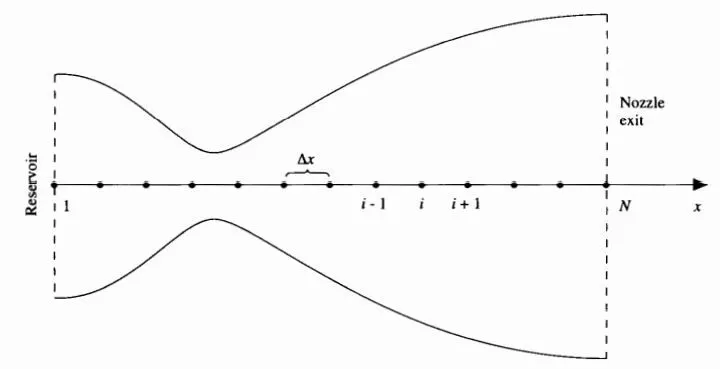
- The first grid point, labeled point 1, is assumed to be in the reservoir. The points are evenly distributed along the x-axis, with `Deltax` denoting the spacing between grid points. The last point, namely, that at the nozzle exit, is denoted by N; we have a total number of N grid points distributed along the axis.
-Point i is simply an arbitrary grid point, with points i - 1 and i + 1 as the adjacent points.
2. Discretization of Equation- By using Mac-Cormack's technique
MacCormack's technique is a predictor-corrector method in the time-marching approach, as we know the flow-field variables at time t, and we use the difference equations to solve explicitly for the variables at time `t + Deltat`
Predicto step- by doing Forward Differencing we calculate for,
`((del rho)/(del t))_i^t` , `((del V)/(del t))_i^t` and `((delT)/(del t))_i^t`
Solution update- Now we calculate the Predicted values
`barrho_i^(t+Deltat) = rho_i^t + ((del rho)/(del t))_i^t Deltat`
`barV_i^(t+Deltat) = V_i^t + ((del V)/(del t))_i^t Deltat`
`barT_i^(t+Deltat) =T_i^t + ((del T)/(del t))_i^t Deltat`
Corrector step- we do Backward differencing in this step using the predicted values
`((bar(del rho))/(del t))_i^(t+Deltat)` , `((bar(del V))/(del t))_i^(t+Deltat)` and `((bar(del T))/(del t))_i^(t+Deltat)`
Average solution - Now the average time derivatives will be,
`((del rho)/(del t))_(avg) = 0.5[((del rho)/(del t))_i^t + (bar(del rho)/(delt))_i^(t+Deltat)]`
`((del V)/(del t))_(avg) = 0.5[((del V)/(del t))_i^t + (bar(del V)/(delt))_i^(t+Deltat)]`
`((del T)/(del t))_(avg) = 0.5[((del T)/(del t))_i^t + (bar(del T)/(delt))_i^(t+Deltat)]`
Finally, we have for the Actual values(corrected values) of the flow-fieald variables at time `t+Deltat`
`rho_i^(t+Delta t) = rho_i^t + ((del rho)/(del t))_(avg) Deltat`
`V_i^(t+Delta t) = V_i^t + ((del V)/(del t))_(avg) Deltat`
`T_i^(t+Delta t) = T_i^t + ((del T)/(del t))_(avg) Deltat`
- All the variables in are the nondimensional values. Also, eqations constitute our second eschelon of equations.
- The finite-difference expressions of the governing equations in a form that pertains to MacCormack's technique.
3. Calculation of Time Step
In this solution magnitude of the time step is calculated based on the Courant number(C).
The simple stability analysis of linear hyperbola equations gives the result that C < 1 for an explicit numerical solution, gives a stable solution.
- The magnitude of dt is calculated by using the formula,
`Deltat = C (Deltax)/(a+V)`
- CFL for a one-dimensional flow, where 'V' is the local flow velocity at a point in the flow and 'a' is the local speed of sound
- With the help of the above formula, the value of dt is calculated at each node. Once, after calculating the dt value at all the nodes minimum of all dt is considered.
4. Boundary Conditions
- It is an all-important aspect because, without the physically proper implementation of boundary conditions and their numerically proper representation, we have no hope whatsoever of obtaining a proper numerical solution to our flow problem
- Point 1 is essentially in the reservoir it represents an inflow boundary, with the flow coming from the reservoir and entering the nozzle. In contrast, point N is an outflow boundary, with flow leaving the nozzle at the nozzle exit. Moreover, the flow velocity at point 1 is a very low, subsonic value
At the inlet, Since point 1 is viewed as essentially the reservoir, we stipulate the density and temperature at point 1 to be their respective stagnation values, Po and To, respectively the flow variables such as temperature and density remain constant, and the value of velocity changes.
To find V1 by linear extrapolation, we have
`V_1 = 2V_2 - V_3`
At the outlet, Supersonic outflow boundary (point N), all the flow variables keep on changing, again use linear extrapolation based on the flow-field values at the internal points,
`V_N = 2V_(N-1) - V_(N-2)`
`rho_N = 2rho_(N-1) - rho_(N-2)`
`T_N = 2T_(N-1)-T_(N-2)`
Nozzle shape & Initial conditions
The nozzle shape, A = A(x) is specified and held fixed, independent of time, we choose parabolic area distribution given by:
`A = 1 + 2.2(x-1.5)^2` `0lexle3`
We know that p and T decrease and V increase as the flow expands through the nozzle. Hence, we choose initial conditions that qualitatively behave in the same fashion.
For simplicity, let us assume linear variations of the flow-field variables, as a function of x, Than initial condition at t=0
`rho = 1 - 0.3146x`
`T = 1 - 0.2314x`
`V = (0.1 + 1.09x)T^(1/2)`
5. A Computer Program below is made to solve the Quasi 1D Nozzle Flow For Non-Conservative Form
MATLAB Program:- Non-Conservative Form
clear all
close all
clc

% Inputs
n = 31; % Grid Points As published in John D Anderson Book
x = linspace(0,3,n);
dx = x(2)-x(1);
gamma = 1.4;

% Throat Grid Point
th = round(n/2);

% Calculate Initial Profiles
rho = 1 - 0.3146*x;
t = 1 - 0.2314*x; % t = temperature
v = (0.1 + 1.09*x).*t.^0.5;

%cfl = 1 for Convection || [max((v+sqrt(t))*dt/dx)]
cfl = 1;

% area
a = 1 + 2.2*(x - 1.5).^2;

% Time Step
nt = 1400;
dt = cfl*dx/max(v+sqrt(t));


% Outer time loop
for k = 1:nt

    % Copy Of values
    rho_old = rho;
    v_old = v;
    t_old = t;

    % Predictor method

    for j = 2:n-1
        % drho_dt_p = -rho(j)*(v(j+1)-v(j))/dx - rho(j)*v(j)*(log(a(j+1)-log(a(j)))/dx - v(i)*(rho(j+1)-rho(j))/dx
        dvdx = (v(j+1)-v(j))/dx;
        drhodx = (rho(j+1)-rho(j))/dx;
        dtdx = (t(j+1)-t(j))/dx;
        dlog_adx = (log(a(j+1))-log(a(j)))/dx;

        % Continuity Equation
        drhodt_p(j) = -rho(j)*dvdx - rho(j)*v(j)*dlog_adx - v(j)*drhodx;

        % Momentum Equation
        dvdt_p(j) = -v(j)*dvdx - (gamma^-1)*(dtdx + (t(j)/rho(j))*drhodx);

        % Energy
        dtdt_p(j) = -v(j)*dtdx - (gamma-1)* t(j)*(dvdx + v(j)*dlog_adx);

        % Solution Update
        rho(j) = rho(j) + drhodt_p(j)*dt;
        v(j) = v(j) + dvdt_p(j)*dt;
        t(j) = t(j) + dtdt_p(j)*dt;

    end

    % Corrector method

    for j = 2:n-1
        dvdx = (v(j)-v(j-1))/dx;
        drhodx = (rho(j)-rho(j-1))/dx;
        dtdx = (t(j)-t(j-1))/dx;
        dlog_adx = (log(a(j))-log(a(j-1)))/dx;

        % Continuity Equation
        drhodt_c(j) = -rho(j)*dvdx - rho(j)*v(j)*dlog_adx - v(j)*drhodx;

        % Momentum Equation
        dvdt_c(j) = -v(j)*dvdx - (gamma^-1)*(dtdx + (t(j)/rho(j))*drhodx);

        % Energy
        dtdt_c(j) = -v(j)*dtdx - (gamma-1)* t(j)*(dvdx + v(j)*dlog_adx);

    end

    % Compute Average Time Derivative
    drhodt = 0.5*(drhodt_p + drhodt_c);
    dvdt = 0.5*(dvdt_p + dvdt_c);
    dtdt = 0.5*(dtdt_p + dtdt_c);

    for  i = 2:n-1
    % Final Solution update
    rho(i) = rho_old(i) + drhodt(i)*dt;
    v(i) = v_old(i) + dvdt(i)*dt;
    t(i) = t_old(i) + dtdt(i)*dt;

    end

    % Apply Boundary Condition
    % Inlet
    v(1) = 2*v(2) -  v(3);

    % Outlet
    rho(n) = 2*rho(n-1) - rho(n-2);
    v(n) = 2*v(n-1) - v(n-2);
    t(n) = 2*t(n-1) - t(n-2);


    % Pressure
    p = rho.*t;
    % Mach Number (Speed Of Sound = 340m/s)
    % M = V/A || (Velocity of Object/Velocity of Sound)
    % A = sqrt(gamma*r*t) || where;- gamma=1.4, r=gas constant, t = temmperature
    % Assume;- (gamma=1,r=1) for the sake of simplicity of code
    M = v./sqrt(t);
    % Mass Flow Rate
    m = rho.*a.*v;


    % Plots for Variation of Mass Flow Rate at Different Time Step
    figure(4)
    hold on
    if k ==1
        plot(x,m)
    end
    if k ==50
        plot(x,m)
    end
    if k ==250
        plot(x,m)
    end
    if k ==500
        plot(x,m)
    end
    if k ==750
        plot(x,m)
    end
    if k ==1000
        plot(x,m)
    end

    % Primitive Variable Profiles at Throat || th = 16
    rho_throat(k) = rho(th);
    v_throat(k) = v(th);
    t_throat(k) = t(th);
    p_throat(k) = p(th);
    M_throat(k) = M(th);


end

xlabel('Nozzle Length')
ylabel('Mass Flow Rate')
legend('1dt','50dt','250dt','500dt','750dt','1400dt')
title('Variation of Mass Flow Rate at Different Time Step')

% Plots For Steady State Primitive Variable Profiles
figure(1)
subplot(5,1,1)
plot(x,v)
xlabel('Nozzle Length')
ylabel('Velocity')
title('Steady State Primitive Variable Profiles')
subplot(5,1,2)
plot(x,rho)
xlabel('Nozzle Length')
ylabel('Density')
subplot(5,1,3)
plot(x,t)
xlabel('Nozzle Length')
ylabel('Temperature')
subplot(5,1,4)
plot(x,p)
xlabel('Nozzle Length')
ylabel('Pressure')
subplot(5,1,5)
plot(x,M)
xlabel('Nozzle Length')
ylabel('Mach Number')

% Plots For Transient Variation of Primitive Variable at Throat
figure(2)
subplot(5,1,1)
plot(v_throat)
xlabel('Time Step')
ylabel('Velocity')
title('Transient Variation of Primitive Variable at Throat')
subplot(5,1,2)
plot(rho_throat)
xlabel('Time Step')
ylabel('Density')
subplot(5,1,3)
plot(t_throat)
xlabel('Time Step')
ylabel('Temperature')
subplot(5,1,4)
plot(p_throat)
xlabel('Time Step')
ylabel('Pressure')
subplot(5,1,5)
plot(M_throat)
xlabel('Time Step')
ylabel('Mach Number')

% Plot For Steady State Mass Flow Rate Profiles
figure(3)
plot(x,m)
xlabel('Nozzle Length')
ylabel('Mass Flow Rate')
title('Steady State Mass Flow Rate Profiles')
Output:-
# Non-conservative form
1. Plots for Steady-state distribution of the Primitive variables inside the nozzle
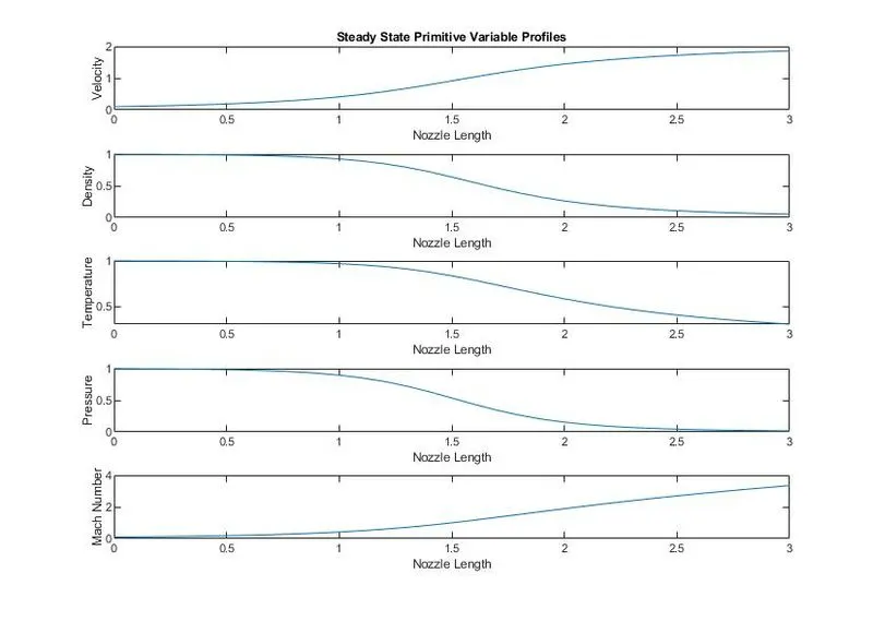
- After 1400 time steps, the numerically calculated primitive variables are converged to the exact analytical solution.
- Initially, some primitive variables were set to the initial condition and, others were allowed to float as a part of the inflow subsonic boundary condition.
- At n = 1, the non-dimensional pressure or pressure ratio (`p/p_0`) of the fluid element was set to 1 (reservoir end), then as a part of the numerical explicit scheme (MacCormack method), the pressure variations were calculated as a function of time along with the nozzle. There is a decrease in the pressure as the flow changes from the subsonic state(convergent, M<1) to sonic state(throat, M=1) and similarly from sonic (throat, M=1) to supersonic state(divergent, M>1).
- Velocity of the fluid will increase traveling through convergent (subsonic)`implies` throat(sonic)`implies` divergent section(supersonic). Similarly, as the velocity increases, the Mach number will increase accordingly as a function of the length of the nozzle.
- Similar is the case for density and temperature. The pressure difference present inside the system and in the surrounding is responsible for the fluid flow. This pressure difference (reservoir and exit/surrounding) gradually decreases as a function of the time and length of the nozzle as the fluid travels towards the exit of the divergent section.
2. Plots for Transient-state distribution of the Primitive variables at the throat
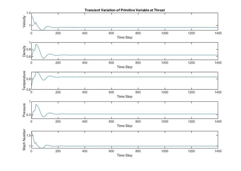
- The above plots show the time-wise variation of the flow-field variables i.e. Density, Velocity, Temperature, Pressure, Mach number, plotted versus the number of time steps. The x-axis is a time axis that starts at zero and ends at time step 1400.
- Note that the largest changes take place at early times, after which the final, steady-state value is approached almost asymptotically.
3. Variation of Mass flow rate distribution inside the nozzle at different time steps-
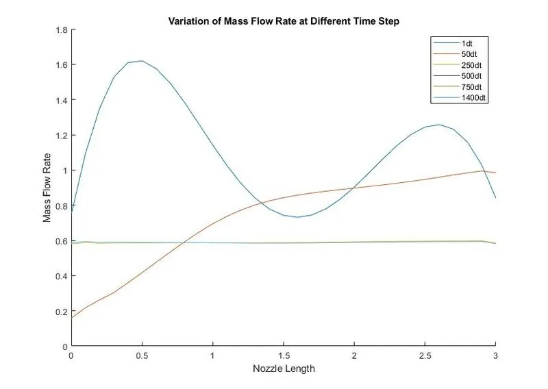
- Time-wise variation of the flow and its approach to the steady-state is provided by the mass flow variations shown in the above fig. Here the non-dimensional mass flow (ρ A V) is plotted as a function of nondimensional distance through the nozzle.
- Five different curves are shown, each for a different time during the course of the time-marching procedure. After 50 time steps, the mass flow distribution through the nozzle changed considerably. After 100 time steps, the mass flow distribution has changed radically; the mass flow variation is simply flopping around inside the nozzle due to the transient variation of the flow field variables. however, after 200 time-steps, the mass flow distribution is beginning to settle down, and after 700 time-steps, the mass flow distribution is a straight, horizontal line across the graph. This says that the mass flow has converged to a constant, steady-state value throughout the nozzle.
____________________________________________________________________________________________________________
-------------------------------------------------------------------------------------------------------------------------------------------------
# Conservation Forms: Conservation equation for one-dimensional inviscid flow,
Continuity equation
`(del(rho A))/(del t) + (del(rho A V))/(del x) =0`
Momentum equation
`(del(rho AV))/(del t) + (del(rho A V^2))/(del x) = -A (del p)/(del x)`
Energy Equation
`(del(rho(e+V^2/2)A))/(del t) +(del (rho(e+V^2/2)AV))/(del x) = - (del(rho A V))/(del x)`
In terms of Non-Dimensional forms Above governing equation in terms of non-dimensional variables
Continuity equation
`(del(rho^' A^'))/(del t^') + (del(rho^' A^' V^'))/(del x^') = 0`
Momentum equation
`(del (rho^' A^' V^'))/(delt^') + (del(rho^' A^'V^' + (1/gamma) p^'A^'))/(delx^') = 1/gamma p^' (del A^')/(del x^')`
Energy Equation
`(del[rho^'((e^')/(gamma-1) + gamma/2 V^('2))A^'])/(del t^') + (del[rho^'((e^')/(gamma-1) + gamma/2 V^('2))V^'A^' + p^' A^' V^'])/(delx^') = 0`
- Above are the nondimensional conservation form of the continuity, momentum, and energy equations for quasi-one-dimensional flow, respectively.
- Lets express the equations for the quasi-one-dimensional flow in more generic form. We're going to define the solution vector U, the flux vector F, and the source term J as follows:
`U_1 = rho^' A^'`
`U_2 = rho^' A^' V^'`
`U_3 = rho^' ((e^')/(gamma-1) + gamma/2 V^('2) ) A^'`
`F_1= rho^' A^' V^'`
`F_2= rho^' A^' V^('2) + 1/gamma rho^' A^'`
`F_3 = rho^'((e^')/(gamma-1) + gamma/2 V^('2))V^'A^' + p^'A^' V^'`
`J_2 = 1/gamma p^' (delA^')/(del x^')`
With these above element equation we can write our Non-Dimensional forms of governing equation as,
`(del U_1)/(del t^') = - (del F_1)/(del x^')`
`(del U_2)/(del t^') = - (del F_2)/(del x^') + J_2`
`(del U_3)/(del t^') = - (del F_3)/(del x^')`
- Now as we know in conservation form of the equations the dependent variables(the variables for which we directly obtain numbers) are not the primitive variables.
- Now, to obtain primitive variables(`rho`,V,T, P,etc) we must decode the elements U1,U2 & U3 as follows, we have,
`rho^' = U_1/A^'`
`V^' = U_2/U_1``T^' = e^' = (gamma-1) (U_3/U_1 - gamma/2 V^('2))`
`p^' = rho^' T^'`
In the above equations, we can notice that the flux vector elements F1, F2 & F3 are source terms couched in terms of the primitive variables if we directly use F1, F2 & F3 in the Computer Program in terms of `rho^', V^',p^' and e^'` instabilities develop during the course of time-marching solution.
So, we write such that the governing equations are in pure form in terms of the elements of the solution vector i.e in terms of(`U_1, U_2, U_3`) , and avoid the use of primitive variable
Pure Form of the Flux terms, consider the flux term `F_1`, than
`F_1 = U_2`
`F_2 = U_2^2/U_1 + (gamma-1)/gamma(U_3-gamma/2 U_2^2/U_1)`
`F_3 = gamma (U_2U_3)/U_1 - (gamma(gamma-1))/2 U_2^3/U_1^2`
`J_2 = (gamma-1)/gamma (U_3-gamma/2 U_2^2/U_1^2) (del(ln A^'))/(del x^')`
This is the 'pure' form of the governing equation in conservation form, so solving it on computer program the solution will be stable and converge to a steady state.
Steps to solve the above Governing equation-
1. Meshing- we divide the x-axis along with the nozzle into uniform discrete grid points, same as done in Non-Conservative Form
3. Calculation of Time Step - We follow the same step for Time Step as performed for Non-Conservative Form
- In this solution magnitude of the time step is calculated based on the Courant number(C).
- The magnitude of dt is calculated by using the formula,
`Deltat = C (Deltax)/(a+V)`
2. Apply Boundary Condition- The boundary conditions for the subsonic-supersonic isentropic flow solution using the conservation form of the governing equations are theoretically the same as discussed in the Boundary Conditions at the subsonic inflow boundary.
The nozzle's shape, A = A(x), is specified and held fixed, independent of time. For the case illustrated in this section, we're choosing a parabolic area distribution given by:
`A = 1 + 2.2(x-1.5)^2` `0lexle3`
The Subsonic Inflow boundary condition at Point 1
At the subsonic inflow boundary, two properties are held fixed and one is allowed to float, we hold p' and T' fixed at the inflow boundary, both equal to 1.0, and allow V' to float.
By holding p' fixed, then U1 at grid point i = 1 is fixed, independent of time, via U1 = p 'A', i.e
`U_(1(i=1)) = (rho^' A^')_(i=1) = A_(i=1)^' =`fixed value
The floating value of V' at the inflow boundary is calculated at the end of each time step by linearly extrapolating U2 from the known values at the internal grid point i = 2 and 3, that is,
`U_(2(i=1)) = 2U_(2(i=2))-U_(2(i=3))`
Since V' floats at the inflow boundary, so does the value of U3, which is given by
`U_3 = U_1(T^'/(gamma-1) + gamma/2 V^('2))`
The Supersonic outflow boundary condition at Point N
At the supersonic outflow boundary, all properties are allowed to float. The flow properties at the downstream, supersonic outflow boundary are obtained by linear extrapolation from the two adjacent internal points. If N denotes the grid point at the outflow boundary, then
`(U_1)_N = 2(U_1)_(N-1) - (U_1)_(N-2)`
`(U_2)_N = 2(U_2)_(N-1) - (U_2)_(N-2)`
`(U_3)_N = 2(U_3)_(N-1) - (U_3)_(N-2)`
Initial Condition- Since the dependent variables being solved are U1, U2, and U3, we need initial conditions for these same variables at time t = 0 in order to start the finite-difference solution. The initial conditions for U1, U2, and U3 will also allow initial conditions for F1, F2 & F3 to be obtained from the above equations. Such initial conditions for F1, F2 & F3 are needed to form the x derivatives on the right-hand sides of the governing equations at the first time step.
The initial conditions for U1, U2, and U3 were synthesized by assuming the following variations for `rho^'` & `T^'`
for `0 le x^' le 0.5`
`rho^' = 1`
`T^' = 1`
for `0.5 le x^' le 1.5`
`rho^' =1-0.366(x^'-0.5)`
`T^' =1-0.167(x^'-0.5)`
for `1.5 le x^' le 3.5`
`rho^' = 0.634 - 0.3879(x^'-1.5)`
`T^' = 0.833 - 0.3507(x^'-1.5)`
3. Discretization of Equation- By using Mac-Cormack's technique
Finally, we're now going to discretize the governing equations that consist of flux terms and source terms by using MacCormack's Method.
Predictor step- by doing Forward Differencing we calculate for,
`((del U_1)/(del t^'))_i^(t^')` , `((del U_2)/(del t^'))_i^(t^')` and `((del U_3)/(del t^'))_i^(t^')`
Solution update- Now we calculate the Predicted values
`(barU_1)_i^(t^'+Deltat^') = (U_1)_i^(t^') + ((del U_1)/(del t^'))_i^(t^') Deltat^'`
`(barU_2)_i^(t^'+Deltat^') = (U_2)_i^(t^') + ((del U_2)/(del t^'))_i^(t^') Deltat^'`
`(barU_3)_i^(t^'+Deltat^') = (U_3)_i^(t^') + ((del U_3)/(del t^'))_i^(t^') Deltat^'`
Corrector step- we do Backward differencing in this step using the predicted values
`((bar(del U_1))/(del t^'))_i^(t^'+Deltat^')`
`((bar(del U_2))/(del t^'))_i^(t^'+Deltat^')`
`((bar(del U_3))/(del t^'))_i^(t^'+Deltat^')`
Average solution - Now the average time derivatives will be,
`((del U_1)/(del t))_(avg) = 0.5[((del U_1)/(del t^'))_i^(t^') + (bar(del U_1)/(delt^'))_i^(t^'+Deltat^')]`
`((del U_2)/(del t))_(avg) = 0.5[((del U_2)/(del t^'))_i^(t^') + (bar(del U_2)/(delt^'))_i^(t^'+Deltat^')]`
`((del U_3)/(del t))_(avg) = 0.5[((del U_3)/(del t^'))_i^(t^') + (bar(del U_3)/(delt^'))_i^(t^'+Deltat^')]`
Finally, we have for the Actual values(corrected values) of the flow-fieald variables at time `t+Deltat`
`(U_1)_i^(t^'+Delta t^') = (U_1)_i^(t^') + ((del U_1)/(del t^'))_(avg) Deltat`
`(U_2)_i^(t^'+Delta t^') = (U_2)_i^(t^') + ((del U_2)/(del t^'))_(avg) Deltat`
`(U_3)_i^(t^'+Delta t^') = (U_3)_i^(t^') + ((del U_3)/(del t^'))_(avg) Deltat`
The final corrected values of U1 , U2 , and U3 at time step `t^'+Deltat^'` (here, since t' = O to start with, we are calculating the final corrected values at time `t^'=Deltat^'`') are obtained from
`(rho^')_i^(t^'+Delta t^') = (U_1)_i^(t^'+Delta t^')`
`(V^')_i^(t^'+Delta t^') = (U_2/U_1)_i^(t^'+Delta t^')`
`(T^')_i^(t^'+Delta t^') = (gamma-1) (U_3/U_1 - gamma/2 V^('2))_i^(t^'+Delta t^')`
- This process is repeated for all the interior grid points distributed along with the nozzle, The properties at the inflow and outflow boundaries are calculated as described in the Boundary Conditions
4. A Computer Program below is made to solve the Quasi 1D Nozzle Flow For Conservative Form
MATLAB Program:- Conservative Form
clear all
close all
clc

% Inputs
n = 31; % Grid Points As published in John D Anderson Book
x = linspace(0,3,n);
dx = x(2)-x(1);
gamma = 1.4;

% Throat Grid Point
th = round(n/2);

% % Calculate Initial Profiles
% rho = 1 - 0.3146*x;
% t = 1 - 0.2314*x; % t = temperature
% v = (0.1 + 1.09*x).*t.^0.5;

for i = 1:n
    if x(i) <= 0.5
       rho(i) = 1;
       t(i) = 1;
    end

    if x(i) > 0.5 && x(i) <= 1.5
        rho(i) = 1 - 0.366*(x(i)-0.5);
        t(i) = 1 - 0.167*(x(i)-0.5);
    end

    if x(i) > 1.5
       rho(i) = 0.634 - 0.3879*(x(i)-1.5);
       t(i) = 0.833 - 0.3507*(x(i)-1.5);
    end


end

% Area
a = 1 + 2.2*(x - 1.5).^2;

v = 0.59./(rho.*a);


%cfl = 1 for Convection || [max((v+sqrt(t))*dt/dx)]
cfl = 1;

% Time Step
nt = 1400;
dt = cfl*dx/max(v+sqrt(t));

%dt = 0.0267 %% In John D Anderson book
%cfl = max((v+sqrt(t))*dt/dx)

U1 = rho.*a;
U2 = rho.*a.*v;
U3 = U1.*(t/(gamma-1) + (gamma/2)*v.^2);


% Outer time loop
for k = 1:nt

    % Copy Of values
    U1_old = U1;
    U2_old = U2;
    U3_old = U3;

    % Flux Variables
    F1 = U2;
    F2 = U2.^2./U1 + ((gamma-1)/gamma)*(U3 - (gamma/2)* (U2.^2./U1));
    F3 = gamma*U2.*U3./U1 - 0.5*gamma*(gamma-1)* (U2.^3./U1.^2);


    % Predictor method

    for j = 2:n-1

        % Continuity Equation
        dU1dt_p(j) = -(F1(j+1) - F1(j))/dx;

        J2 = (1/gamma)*rho(j)*t(j)*(a(j+1)-a(j))/dx;

        % Momentum Equation
        dU2dt_p(j) = -(F2(j+1) - F2(j))/dx + J2;

        % Energy
        dU3dt_p(j) = -(F3(j+1) - F3(j))/dx;

        % Solution Update
        U1(j) = U1(j) + dU1dt_p(j)*dt;
        U2(j) = U2(j) + dU2dt_p(j)*dt;
        U3(j) = U3(j) + dU3dt_p(j)*dt;


    end

    % Predictor Update
    rho = U1./a;
    t = (gamma-1)*(U3./U1 - (gamma/2)*(U2./U1).^2);

    % Recalculate The Flux Term
    F1 = U2;
    F2 = U2.^2./U1 + ((gamma-1)/gamma)*(U3 - (gamma/2)* (U2.^2./U1));
    F3 = gamma*U2.*U3./U1 - 0.5*gamma*(gamma-1)* (U2.^3./U1.^2);

    % Corrector method

     for j = 2:n-1

        % Continuity Equation
        dU1dt_c(j) = -(F1(j) - F1(j-1))/dx;

        J2 = (1/gamma)*rho(j)*t(j)*(a(j)-a(j-1))/dx;

        % Momentum Equation
        dU2dt_c(j) = -(F2(j) - F2(j-1))/dx + J2;

        % Energy
        dU3dt_c(j) = -(F3(j) - F3(j-1))/dx;


     end

    % Compute Average Time Derivative
    dU1dt = 0.5*(dU1dt_p + dU1dt_c);
    dU2dt = 0.5*(dU2dt_p + dU2dt_c);
    dU3dt = 0.5*(dU3dt_p + dU3dt_c);

    % Final Solution update
    for  i = 2:n-1
    U1(i) = U1_old(i) + dU1dt(i)*dt;
    U2(i) = U2_old(i) + dU2dt(i)*dt;
    U3(i) = U3_old(i) + dU3dt(i)*dt;

    end

    % Final Update
    rho = U1./a;
    t = (gamma-1)*(U3./U1 - (gamma/2)*(U2./U1).^2);
    v = U2./U1;

    % Apply Boundary Condition
    % Inlet
    U1(1) = a(1);
    U2(1) = 2*U2(2) - U2(3);
    U3(1) = U1(1)*(t(1)/(gamma-1) + 0.5*gamma*v(1)^2);

    % Outlet
    U1(n) = 2*U1(n-1) - U1(n-2);
    U2(n) = 2*U2(n-1) - U2(n-2);
    U3(n) = 2*U3(n-1) - U3(n-2);


    % Pressure
    p = rho.*t;
    % Mach Number (Speed Of Sound = 340m/s)
    % M = V/A || (Velocity of Object/Velocity of Sound)
    % A = sqrt(gamma*r*t) || where;- gamma=1.4, r=gas constant, t = temmperature
    % Assume;- (gamma=1,r=1) for the sake of simplicity of code
    M = v./sqrt(t);
    % Mass Flow Rate
    m = rho.*a.*v;


    % Plots for Variation of Mass Flow Rate at Different Time Step
    figure(4)
    hold on
    if k ==1
        plot(x,m)
    end
    if k ==50
        plot(x,m)
    end
    if k ==250
        plot(x,m)
    end
    if k ==500
        plot(x,m)
    end
    if k ==750
        plot(x,m)
    end
    if k ==1000
        plot(x,m)
    end

    % Primitive Variable Profiles at Throat || th = 16
    rho_throat(k) = rho(th);
    v_throat(k) = v(th);
    t_throat(k) = t(th);
    p_throat(k) = p(th);
    M_throat(k) = M(th);


end

xlabel('Nozzle Length')
ylabel('Mass Flow Rate')
legend('1dt','50dt','250dt','500dt','750dt','1400dt')
title('Variation of Mass Flow Rate at Different Time Step')

% Plots For Steady State Primitive Variable Profiles
figure(1)
subplot(5,1,1)
plot(x,v)
xlabel('Nozzle Length')
ylabel('Velocity')
title('Steady State Primitive Variable Profiles')
subplot(5,1,2)
plot(x,rho)
xlabel('Nozzle Length')
ylabel('Density')
subplot(5,1,3)
plot(x,t)
xlabel('Nozzle Length')
ylabel('Temperature')
subplot(5,1,4)
plot(x,p)
xlabel('Nozzle Length')
ylabel('Pressure')
subplot(5,1,5)
plot(x,M)
xlabel('Nozzle Length')
ylabel('Mach Number')

% Plots For Transient Variation of Primitive Variable at Throat
figure(2)
subplot(5,1,1)
plot(v_throat)
xlabel('Time Step')
ylabel('Velocity')
title('Transient Variation of Primitive Variable at Throat')
subplot(5,1,2)
plot(rho_throat)
xlabel('Time Step')
ylabel('Density')
subplot(5,1,3)
plot(t_throat)
xlabel('Time Step')
ylabel('Temperature')
subplot(5,1,4)
plot(p_throat)
xlabel('Time Step')
ylabel('Pressure')
subplot(5,1,5)
plot(M_throat)
xlabel('Time Step')
ylabel('Mach Number')

% Plot For Steady State Mass Flow Rate Profiles
figure(3)
plot(x,m)
xlabel('Nozzle Length')
ylabel('Mass Flow Rate')
title('Steady State Mass Flow Rate Profiles')
Result:-
Conservative form
1. Steady-state distribution of the variables inside the nozzle:
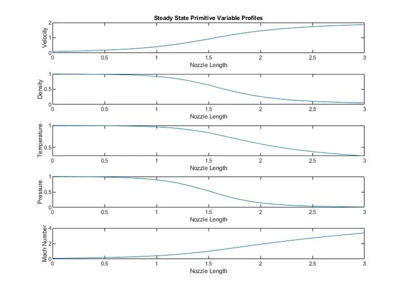
- Here we see that the curves are less smother than the Non-conservative form, the reason behind this is, we are trying to calculate the flux in conservative form and then extracting the primitive variable from these flux terms hence we are rounding off the number therefore we get slightly different value and these errors are small.
2. Time-wise variation of the primitive variables at the nozzle throat (where A = 1)
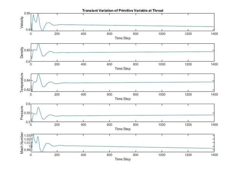
- The graph exhibits the results of time-wise variation of primitives at the nozzle throat, in which, in the approach toward the steady-state solution, at larger values of time( after a large number of time steps), the changes in the flow field variables from one time step to the next become smallest and approach zero in the limit of large time. At this stage, the steady-state has been achieved, and the calculation can be stopped.
- In the non-conservative form we achieve a steady-state for the primitive variable much faster than the conservative form and the reason is the same which is mentioned above.
- Accuracy of the final results in all other parameters, except mass flow rate, is lower in conservative form.
3. Variation of Mass flow rate distribution inside the nozzle at different time steps during the time-marching process
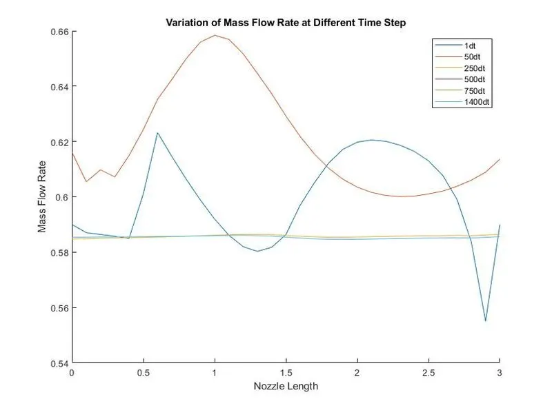
- Time-wise variation of the flow and its approach to the steady-state is provided by the mass flow variations shown in the above figure.
- Five different curves are shown, each for a different time during the course of the time-marching procedure. The result after 50 time-steps, shows a somewhat distribution, after 200 time-steps, the mass flow distribution is becoming more constant, after 700 time-steps it is almost equal to a constant value.
- We observe the graph of mass flow rate with conservative form, and on comparing it with the non-conservative form we found the convergence of curve results are smooth in non-conservative form.
# Comparison of Normalized Mass Flow Rate of both the Forms
clear all
close all
clc

% Inputs
n = 31; % Grid Points
x = linspace(0,3,n);

% Steady State Mass Flow for Non-conservative Froms
mfr_n = [0.587546544935268;0.593833570282515;0.589545249733193;0.590599043115683;0.589591984520660;0.589275345665396;0.588626401670450;0.588027398867411;0.587350692378863;0.586670138783746;0.586002028717861;0.585398632448920;0.584905113040176;0.584563213209041;0.584409723669790;0.584491592888732;0.584857695966768;0.585517571397850;0.586410419420970;0.587426185605423;0.588454832071552;0.589419241366410;0.590279465401973;0.591024989862350;0.591657050862206;0.592197752274650;0.592627997296569;0.593074233163177;0.593143833461227;0.594307495269131;0.581119921196572];
% Steady State Mass Flow for Conservative Forms
mfr_c = [0.585338060151902;0.585419149152737;0.585500269933455;0.585491771734157;0.585541216137707;0.585570690128837;0.585628595503107;0.585688038371644;0.585770884942534;0.585858592482366;0.585959677705216;0.586035825739814;0.586074266333369;0.585989732241028;0.585804167242946;0.585401157984019;0.585080318933882;0.584800918326563;0.584654597779009;0.584626158471301;0.584672137648486;0.584752702451657;0.584841355811849;0.584925863104957;0.584997501861757;0.585064653066355;0.585100003255470;0.585188727267035;0.585094953730803;0.585361020680607;0.585627115947775];


%plotting
plot(x,mfr_n)
hold on
plot(x,mfr_c)
xlabel('Nozzle Length')
ylabel('Mass flow rate')
title('Comparison of Normalized Mass Flow Rate of Both Forms')
legend('Non-conservative','Conservative')
Result-
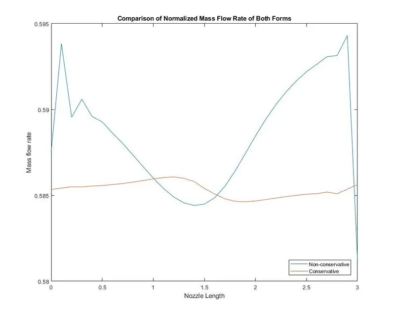
- Here on comparing both the forms we see that the steady-state mass flow distribution predicted by the conservation form is much more satisfactory than that obtained from the nonconservation form.
- The conservation form distribution is much closer to being a constant, while the non-conservation results have a sizable variation at both the inflow and outflow boundary.
- The steady-state mass flow results obtained with the conservation form are on the whole, much closer to the exact analytical solution of `rho*A*V = 0.5844`, shown in the above graph.
- The mass flow rate in both methods, we see that the conservative form gives better result than the non-conservative form because one of the flux terms in the conservative form is the mass flow rate itself therefore we get a better result
- In conservation form takes primary dependant variables and non-conservation form takes secondary dependant variables, so we get a better stable plot for conservation form.
Even though the final solution for both forms is similar, the non-conservative forms oscillate more when compared to the conservative form.
# Grid independence test:
|
Parameters |
Exact analytical solution |
Non-Conservative Form |
Conservative Form |
||
|
n = 31 |
n = 61 |
n = 31 |
n = 61 |
||
|
rho (`rho`) |
0.636 |
0.6396 |
0.6376 |
0.6437 |
0.6375 |
|
T |
0.835 |
0.8368 |
0.8354 |
0.8365 |
0.8347 |
|
p |
0.531 |
0.5353 |
0.5327 |
0.5385 |
0.5321 |
|
Mach number (M) |
1 |
0.9988 |
0.9996 |
0.9942 |
1.006 |
|
Mass Flow Rate (m) |
0.583 |
0.5844 |
0.5826 |
0.5854 |
0.5828 |
- In order to conduct a grid dependency test, here two situations are considered one with 31 grid points and the other with 61 grid point
- From the table, we can observe that as the number of grid points increases the solution accuracy increases and the non-conservative form shows better results than the conservative form.
- It is also clear from the above table that the values are almost the same along with all the primitive variables for both forms even when the grid points are changed from 31 to 61.
So we can conclude that the above problem is Grid independent.
Conclusion:-
- When the Mass flow rate is compared between the two forms. Conservative form is mainly based on the Principle of mass conservation. It is observed the Conservative Form conserves the mass flow rate more than the non-conservative because one of the flux terms in the conservative form is the mass flow rate itself therefore we get a better result
- Upon comparison of both forms we can say there is not much of a difference but the Conservation Form produces better results and stable solutions.
- The error or residual in the Non-Conservative Forms leads to smaller. The convergence state of the solution is obtained in less time because the non-conservative is primarily uses the primitive variables for the solution.
Whereas the Conservative Form uses the solution vector, flux vector to obtain the convergence state of the solution. Processing time increases in converting into the primitive variables. The error or residual increase because of this cause.
- The simulation time for the Non-Conservative Form is shorter than the Conservative Form because the primitive variables converge to a numerical steady-state faster when using the non-conservative form.