Week 7 - Simulation of a 1D Super-sonic nozzle flow simulation using Macormack Method
AIM: To simulate the isentropic flow through a quasi 1D subsonic-supersonic nozzle. Derive both the conservation and non-conservation forms of the governing equations and sovle them using the MacCormack's technique.
OBJECTIVE:
- Solving isentropic flow through a quasi 1D subsonic-supersonic nozzle for conservative and non conservative Method.
- Steady-state distribution of primitive variables inside the nozzle for both the forms.
- To capture the Time-wise variation of flow field primitive variables at the nozzle throat.
- variation of Mass flow rate distribution inside the nozzle at different time steps during the time-marching process
- Comparison of Normalized mass flow rate distributions of both forms.
Theory -with the help of John Anderson COMPUTATIONAL FLUID DYNAMICS- the basics with applications book.
Physical Aspects and the Assumptions of the flow:
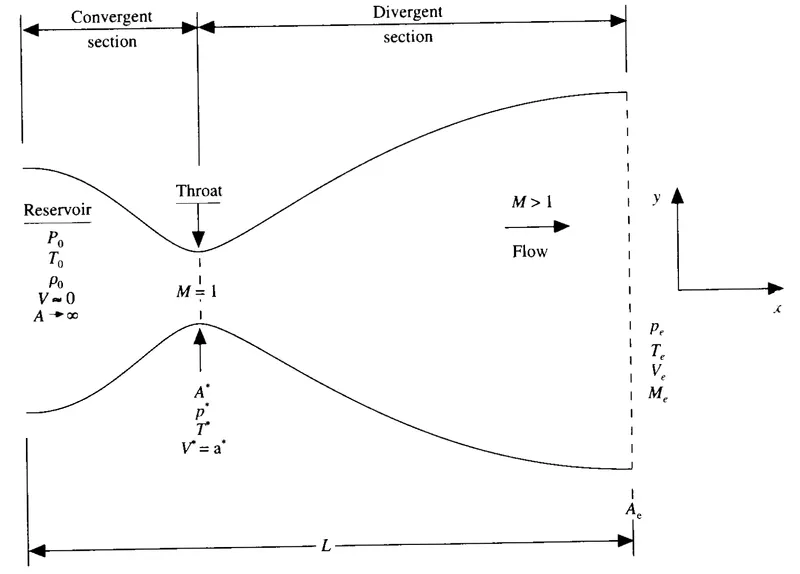
Let we consider the steady, isentropic flow through the convergent- divergent nozzle as given below. The flow at the inlet to the nozzle comes from a reservoir where the pressure and temperature are denoted by p0 , and To, respectively. The cross-sectional area of the reservoir is large ( theoretically, A -- infinity ), and hence thevelocity is very small ( V --0). Thus, Po and T0 are the stagnation values, or total pressure and total temperature, respectively. The flow expands isentropically to supersonic speeds at the nozzle exit, where the exit pressure, temperature, velocity, and Mach number are denoted by Pe, Te, Ve and Me, respectively. The flow is locally subsonic in the convergent section of the nozzle, some at the throat (minimum area), and supersonic at the divergent section. The sonic flow (M = 1) at the throat means that the local velocity at this location is equal to local speed of sound.The 3 important sections we need to be focussed.
- Subsonic where Mach number is less than 1 in the convergent section part of the nozzle.
- Sonic at the throat, where the the local velocity at this location is equal to local speed of sound (denoted by the * )
- Supersonic where the mach number is greater than 1
The expansion goes isentropically.
Assumptions:
We assume that a given section, where the cross-sectional area is A, the flow properties are uniform across that section. Hence, although the area of the nozzle changes as a function of distance along the nozzle, x, and therefore in reality the flow field is two-dimensional (the flow varies in.the two-dimensional .ry space), we make the assumption that the flow properties vary only with x; this is tantamount to assuming uniform flow properties across any given cross section. Such flow is defined as quasi-one-dimensional flow.
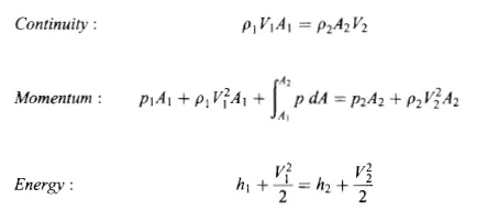
The governing continuity, momentum, and energy equations for this quasi one-dimensional, steady, isentropic flow can be expressed, respectively, as
By solving them analytically we got these graphs shown at below.
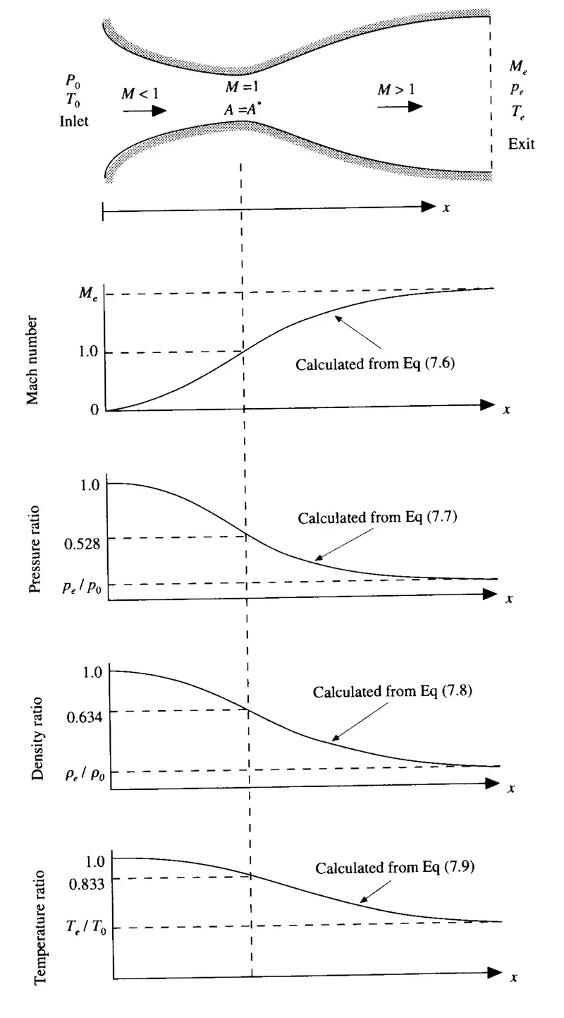
we want to accomplish here is to illustrate the application of various CFD techniques, and we are going to choose a flow problem with a known analytic solution for this illustration.
CFD solution:
The setup
- The governing flow equations will be couched in terms of partial differential equations suitable for the time-marching solution of quasi-one-dimensional flow (the closed-form algebraic equations discussed above are for a steady flow and are not suitable for the present purpose).
- The finite-difference expressions pertaining to MacCormack's technique as applied to this problem will be set up.
- Other details for the numerical solution (such as the calculation of the time stepand the treatment of boundary conditions) will be formulated.
The governing equation can be derived in two forms:
- Conservative form
- Non- conservative form
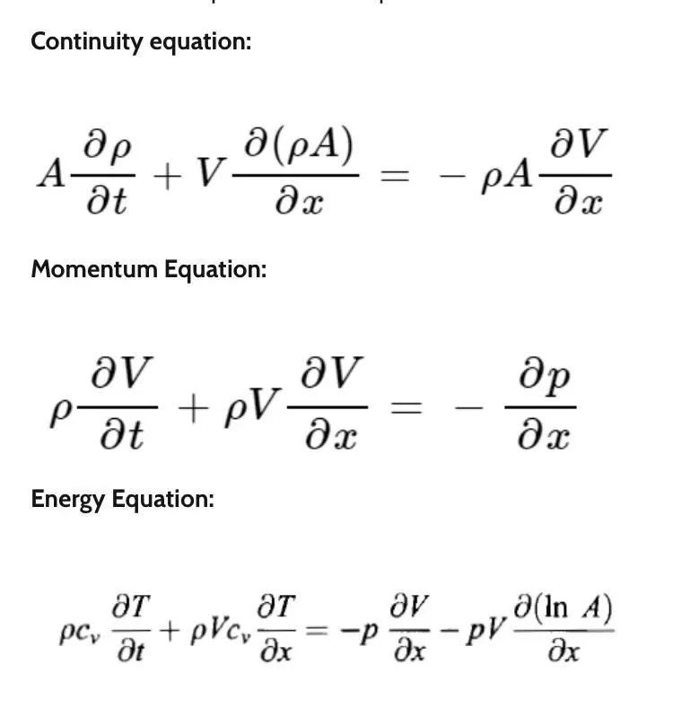
When we apply quasi one dimensional assumptions to these governing equations then we get the equations situable for present problem. The governing equation for quasi- one dimesional are:
- Non- conservative form:
The conservative form of governing equations for quasi 1 D subsonic - supersonic isentropic flow nozzle are
At this stage, we could readily proceed to set up our numerical solution of above equations Note that these are written in terms of dimensional variables. This is fine, and many CFD solutions are carried out directly in terms of such dimensional variables. Indeed, this has an added engineering advantage because it gives you a feeling for the magnitudes of the real physical quantities as the solution progresses. However, for nozzle flows, the flow-field variables are frequently expressed in terms of nondimensional variables,where the flow variables are referenced to their reservoir values. The nondimensional variables p/p0 , p/p0 , and T/T0 vary between O and 1, which is an "aesthetic" advantage when presenting the results. Because fluid dynamicists dealing with nozzle flows so frequently use these nondimensional terms, we will
follow suit here.
here, reservoir temperature and density are denoted by To and p0 , respectively, we define the nondimensional temperature and density, respectively, as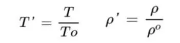
Moreover, L denote the length of the nozzle, we define a dimensionless length as
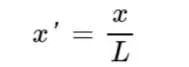
we define a dimensionless velocity as
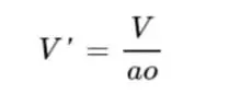
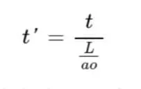
Also, the quantity Liao has the dimension of time, and we define a dimensionless
time as
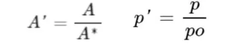
Finally, we ratio the local area A to the sonic throat area A* and define a
dimensionless area as
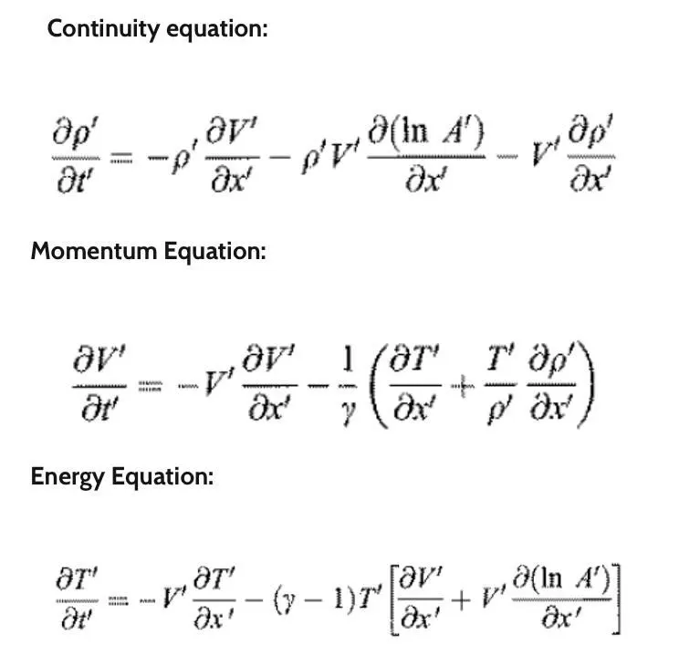
Then we are going to introduce these dimensionless variables we get the non- dimensional governing equations as follows
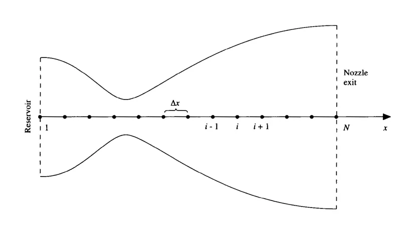
The Finite difference equations: Discretization of equations - Now we are setting up of the finite-difference expressions using MacCormack's explicit technique for the numerical solution of above equations. To implement a finite-difference solution, we divide the x axis along the nozzle into a number of discrete grid points, as shown below (Recall that in our quasi-one-dimensional nozzle assumption, the flow variables across the nozzle cross section at any particular grid point, say point i, are uniform.) the first grid point, labeled point 1, is assumed to be in the reservoir. The points are evenly distributed along the x axis, with dx denoting the spacing between grid points. The last point, namely, that at the nozzle exit, is denoted by N; we have a total number of N grid points distributed along the axis. Point i is simply an arbitrary grid point, with points i - 1 and i + 1 as the adjacent points.
MacCormack's technique is a predictor-corrector method In the time-marching approach, remember that we know the flow-field variables at time t, and we use the difference equations to solve explicitly for the variables at time t + dt.
First, consider the predictor step, In this step we setup the spatial derivatives as forward differences:

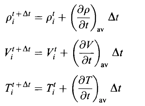
After the predictor step we are proceed with corrector step and then we calculate the time derivates by using these updated values by using backward difference method. Then we calculate the average of the predictor- corrector time derivates.
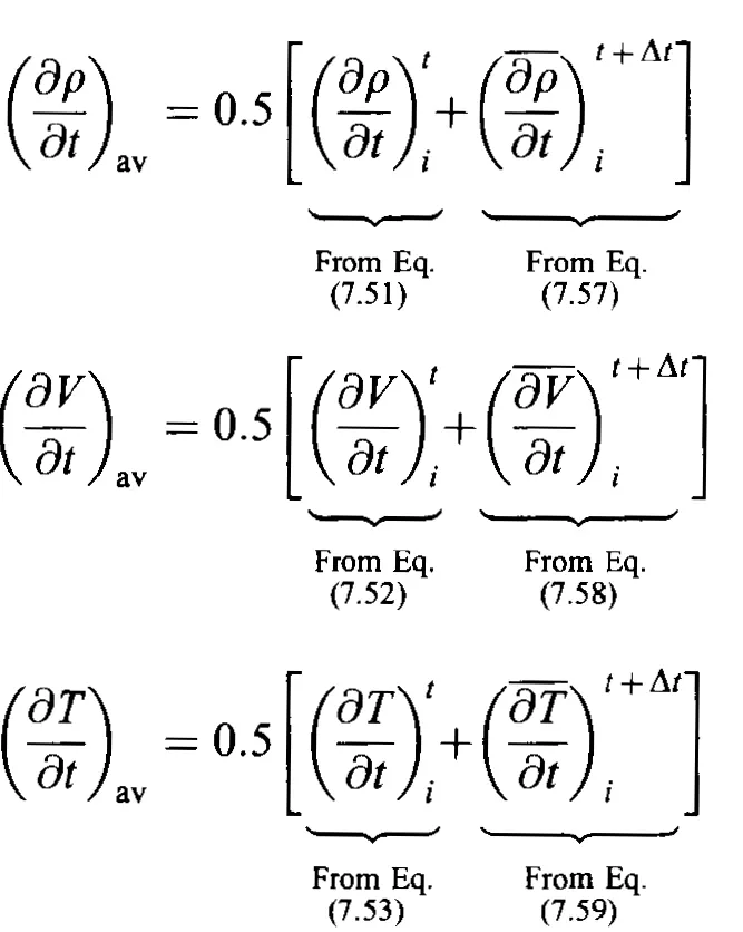
By using this average values we find the corrected values of flow field variables at time t+dt. These steps should be repeated until steady state is reached.
NOZZLE SHAPE AND INITIAL CONDITIONS.
The nozzle shape, A = A(x), is specified and held fixed, independent of time, For the case illustrated in this section, we choose a parabolic area distribution given by
x = 1.5 is the throat of the nozzle, that the convergent section occurs for x < 1.5, and that the divergent section occurs for x > 1.5.
To start the time-marching calculations, we must stipulate initial conditions for p, T, and V as a function of x; that is, we must set up values of p, T and V at time t = O. In theory, these initial conditions can be purely arbitrary.
For the present case we assume the initial conditions for P, T and rho are :

we know that rho and T decrease and V increases as the flow expands through the nozzle. Hence, we choose initial conditions that qualitatively behave in the same fashion. For simplicity, let us assume linear variations of the flow-field variables, as a function of x. For the present case, we assume the following values at time t = 0.
BOUNDARY CONDITIONS:
Another aspect of the numerical solution is that of boundary conditions an all important aspect, because without the physically proper implementation of boundary conditions and their numencally proper representation, we have no hope whatsoever in obtaining a proper numerical solution to our flow problem.
Subsonic inflow boundary (point 1): Here, we must allow one variable to float; we choose the velocity V1, because o~ a physical basis we know the mass flow through the nozzle must be allowed to adJust to the proper steady state, and allowing Vi to throat makes the most sense as part of this adjustment. The value of Vi changes with time and is calculated from information provided by the flow-field solution over the internal points.
The slope of the linear extrapolation line is determmed from points 2 and 3 to calculate V1 and we take rho(1) and T(1) =1 as fixed values.
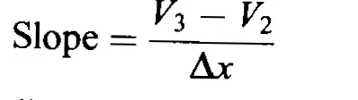
Using this slope to find V1 by linear extrapolation, we have

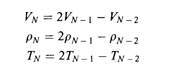
Supersonic outflow boundary (point N): Here, we must allow all flow-field variables to float We again choose to use linear extrapolation based on the flowfield values at the internal points, Specifically, we have, for the nondimensional variables,
Now we write a code by suing this data and do simulation to find out the flow field variables and required data.
2. Conservative form:
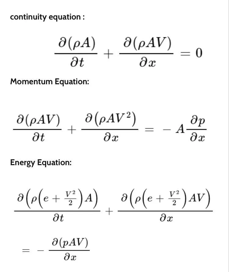
Now converting these equations to non-dimensional form we get the governing equations as:
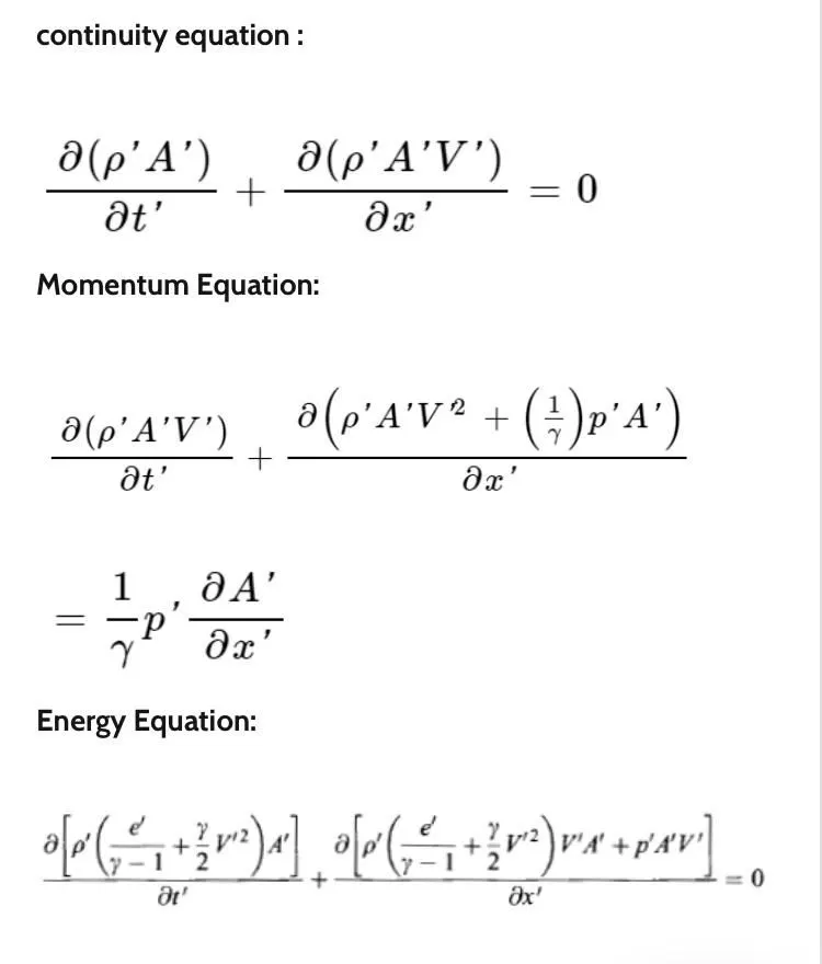
The equations for quasi-onedimensional flow can be expressed in a similar generic form. Let us define the elements of the solutions vector U, the flux vector F, and the source term J as
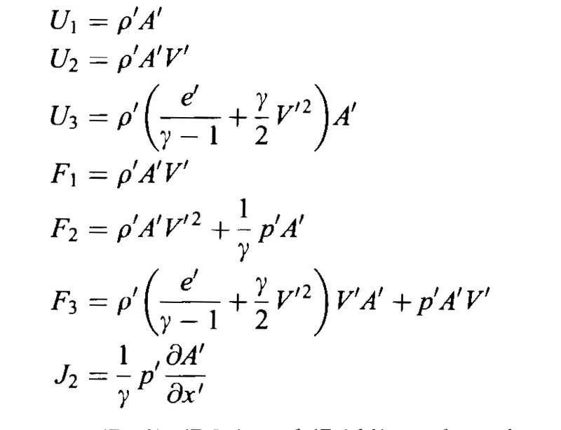
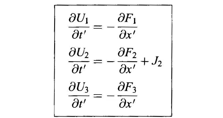
we are writting these equations in the form of as follows:
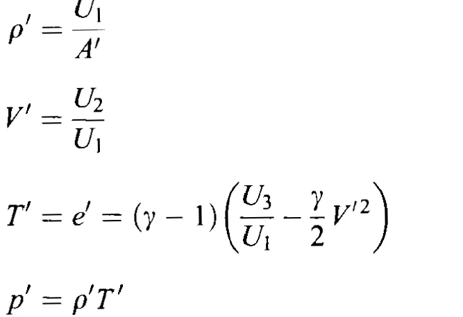
To obtain the primitive variables (rho, V, T, p, etc.), we must decode the elements U1, U2, and U3 as follows. From the definitions of U1 , U2 , and U3 given above, we have
Next we are going to discretization. we take the governing equations that consists of flux terms and source terms and discretize them by using Maccormack's method.
Predictor step:To start the calculation, we use the initial conditions for U1, U2 and U3 to calculate the initial values of F1, F2, and F3 at grid points i = 16 and 17.we use these calculate vaules of U1, U2 and U3 in the next time step. we are calculating time derivatives by using Forward differencing.
Corrector step: Now we are using predicted values to calculate new flux terms and source terms. Then we are calculating time derivates by using Backward differencing. After that we are computing average derivatives of predictor and corrector steps.
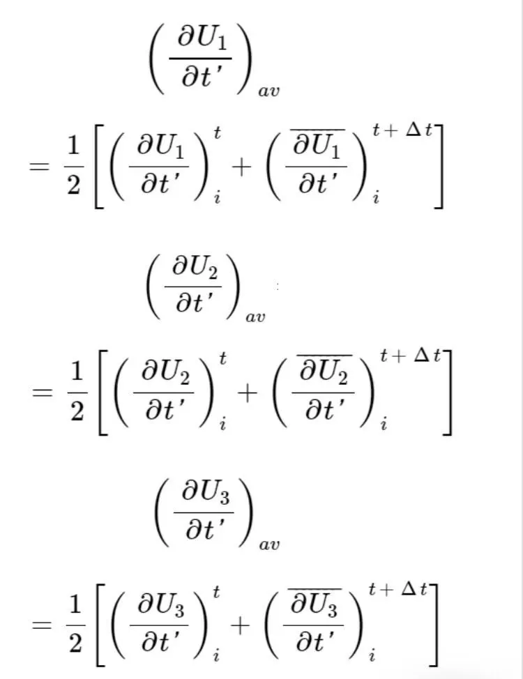
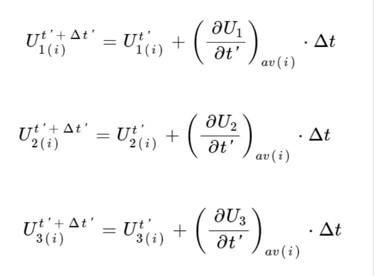
Then we are calculating the corrected values of U1, U2 and U3 by using average values of time derivate. This is done at every node expect the boundary nodes since we calculate them by using boundary conditions and we are also calculate the primitive variables.
Initial conditions and Boundary conditions:
For the present calculations, we choose the following initial conditions, which are qualitatively similar to the final solution. From x' = o to 1.5, we use the same initial conditions as given However, for x > 1.5, we use

These variations slightly more realistic than those assumed in the Nozzle Shape and initial Conditions .This is in anticipation that the stability behavior of the finite difference formulation using the conservation form of the governing equations might be slightly more sensitive, and therefore it is useful to start with more improve initial conditions than those given in Sec. 7.3.1 by Eqs. (7.'.4a) to (7.74c). The initial conditions for the variation of V' is synthesized by taking advantage of the fact that one of the dependent variables in our governing equations, namely U2 is physically the local mass flow; that is, U2 = rho'A'V'. Therefore,for the initialconditions only, let us assume a constant mass flow through the nozzle and calculate V' as
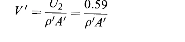
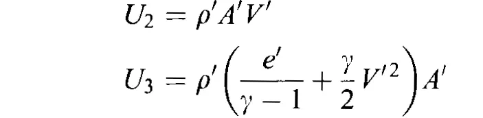
The value 0.59 is chosen for U2 because it is close to the exact analytical value of the steady-state mass flow (which for this case is 0.579). Therefore, the initial condition for V' as a function of x' is obtained by substituting the rho' variation given by Eqs. Finally, the initial conditions for U1 , U2, U3 are obtained by substituting the above variations for rho', T', and V' into the definitions

Boundary conditions:The boundary conditions for the subsonic-supersonic isentropic flow solution using the conservation form of the governing equations are theoretically the same as discussed above
Subsonic Inflow boundary (point1):
subsonic inflow boundary two properties are held fixed and one is allowed to float, and at the supersonic outflow boundary all properties are allowed to float. In the present formulation, as before, we hold rho' and T' fixed at the inflow boundary, both equal to 1, and allow V' to float. By holding ho' fixed, then U1 at grid point i = 1 is fixed, independent of time, via U1 = rho 'A'. That is,

The floating value of V' at the inflow boundary is calculated at the end of each time step by linearly extrapolating U2 from the known values at the internal grid points i = 2 and 3, that is,

and then obtaining V' at i = 1 from Eq. (7 .103 ). Since V' floats at the inflow boundary, so does the value of U3 , which is given by

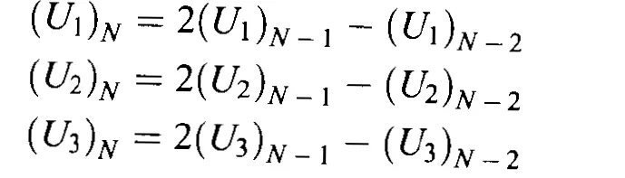
Supersonic outflow boundary:The flow properties at the downstream,supersonic outflow boundary are obtained by linear extrapolation from the two adjacent internal points. If N denotes the grid point at the outflow boundary, then
Grid independence Test:
The numerical solution achieved through CFD is dependent on the grid system adopted. Moreover, the grid spacing also impacts the accuracy and Computational time taken to generate an appreiciable numerical solution. Grid independence test is done to check whether the solution alters from change in the number of grid points (N). If the solution doesnot change with increase in grid points, then the solution is said to be grid independent. In the study we are computing the variable properties on N = 31 and N = 61.
Now, we are writing a code on Matlab/ Octave which solves the quasi 1 D nozzle flow problem using both the methods Conservative and Non- conservative:
Non-Conservative form:-
clear all
close all
clc

%inputs
n = 31;
x = linspace(0,3,n);
dx = x(2) - x(1);
gamma = 1.4;

%calculate initial profiles
rho = 1-0.3146*x;
t = 1-0.2314*x; %t = temperature
v = (0.1+1.09*x).*t.^0.5;

%area
a = 1+2.2*(x-1.5).^2;
%time steps
nt = 1400;
dt = 0.0201; % Time step given in anderson book.

%outer time loop
for k = 1:nt

  rho_old = rho;
  v_old = v;
  t_old = t;

  %predictor method
  for j = 2:n-1
    %define some variables that we are using again and again
    dvdx = (v(j+1)-v(j))/dx;
    drhodx = (rho(j+1)-rho(j))/dx;
    dtdx = (t(j+1)-t(j))/dx;
    dlogadx = (log(a(j+1))-log(a(j)))/dx; % - instead of +

    %continuty equation
    drhodt_p(j) = -rho(j)*dvdx - rho(j)*v(j)*dlogadx - v(j)*drhodx;
    %momentum equation
    dvdt_p(j) = -v(j)*dvdx - (1/gamma)*(dtdx + (t(j)/rho(j))*drhodx);
    %energy equation
    dtdt_p(j) = -v(j)*dtdx - (gamma-1)*t(j)*(dvdx + v(j)*dlogadx);

  endfor

    %solution update
    for j = 2:n-1
    rho(j) = rho(j) + drhodt_p(j)*dt;
    v(j) = v(j) + dvdt_p(j)*dt;
    t(j) = t(j) + dtdt_p(j)*dt;
    endfor

   %corrector method
      for j = 2:n-1
    %define some variables that we are using again and again
    dvdx = (v(j)-v(j-1))/dx;
    drhodx = (rho(j)-rho(j-1))/dx;
    dtdx = (t(j)-t(j-1))/dx;
    dlogadx = (log(a(j))-log(a(j-1)))/dx; % - instead of +

    %continuty equation
    drhodt_c(j) = -rho(j)*dvdx - rho(j)*v(j)*dlogadx - v(j)*drhodx;
    %momentum equation
    dvdt_c(j) = -v(j)*dvdx - (1/gamma)*(dtdx + (t(j)/rho(j))*drhodx);
    %energy equation
    dtdt_c(j) = -v(j)*dtdx - (gamma-1)*t(j)*(dvdx + v(j)*dlogadx);


     endfor

  %compute the average derivates
  drhodt = 0.5*(drhodt_p + drhodt_c);
  dvdt = 0.5*(dvdt_p + dvdt_c);
  dtdt = 0.5*(dtdt_p + dtdt_c);

  %final solution update
   for i = 2:n-1
      rho(i) = rho_old(i) + drhodt(i)*dt;
      v(i) = v_old(i) + dvdt(i)*dt;
      t(i) = t_old(i) + dtdt(i)*dt;

    end

    %apply boundary conditions
    %inlet
    %rho(1) = 2*rho(2) - rho(3);
    %v(1) = 2*v(2) - v(3);          %% Incorrect inlet BC
    %t(1) = 2*t(2) - t(3);

    rho(1) = 1;
    t(1) = 1;
    v(1) = 2*v(2) - v(3);
    %outlet
    rho(n) = 2*rho(n-1) - rho(n-2);
    v(n) = 2*v(n-1) - v(n-2);
    t(n) = 2*t(n-1) - t(n-2);

    %Pressure
    p = rho.*t;
    %Mach no
    M = v./sqrt(t);
    %Mass flow rate
    mf = rho.*a.*v;

    % Variation in throat
    rho_th(k) = rho(16); % 16th node is the throat (mid point) of the nozzle - to check steady state nature
    M_th(k) = M(16);   % as we know, the M at throat is 1  - sonic state
    p_th(k) = p(16);
    t_th(k) = t(16);

  end
    %plotting
    figure(1)
    subplot(4,1,1)
    plot(x,rho)
    xlabel('Nozzle length')
    ylabel('Density')
    title('Steady state variation of primitive variables across the nozzle')
    subplot(4,1,2)
    plot(x,p)
    xlabel('Nozzle length')
    ylabel('Pressure')
    subplot(4,1,3)
    plot(x,M)
    xlabel('Nozzle length')
    ylabel('Mach no')
    subplot(4,1,4)
    plot(x,t)
    xlabel('Nozzle length')
    ylabel('Temperature')

    figure(2)
    subplot(4,1,1)
    plot(rho_th)
    xlabel('Timestep')
    ylabel('Density')
    title('Transient variation of primitive variables at throat')
    subplot(4,1,2)
    plot(p_th)
    xlabel('Timestep')
    ylabel('Pressure')
    subplot(4,1,3)
    plot(M_th)
    xlabel('Timestep')
    ylabel('Mach no')
    subplot(4,1,4)
    plot(t_th)
    xlabel('Timestep')
    ylabel('Temperature')
For Conservative form:-
clear all
close all
clc

%Initialize the domain (x,L,dx)
n = 31;
L = 3;
x = linspace(0,L,n);
dx = x(2)-x(1);
%Area
A = 1+2.2*(x-1.5).^2;
nt = 1400;

%Initial conditions
for i =1:n
  if x(i)<=0.5
    rho(i) = 1;
    t(i) = 1;
  endif
  if x(i)>0.5 && x(i)<=1.5
    rho(i) = 1-0.366*(x(i)-0.5);
    t(i) = 1-0.167*(x(i)-0.5);
  endif
  if x(i)>1.5
    rho(i) = 0.634-0.3897*(x(i)-1.5);
    t(i) = 0.833-0.3507*(x(i)-1.5);
  endif
end
%specific heat capacity
gamma = 1.4;
%Mass flux
U1 = rho.*A;
%Mass flow rate
U2 = 0.59*ones(1,n);
%velocity
v = U2./(rho.*A);
%Energy flux
U3 = rho.*(t/(gamma-1) + gamma*0.5*v.^2).*A;


throat = 16; %16th node

%outer Time loop
for k=1:nt

  %minimum time step
  dt = min((0.5*dx)./(sqrt(t)+v));

  %copies of solution vectors
  U1_old = U1;
  U2_old = U2;
  U3_old = U3;

  %flux terms
   F1 = U2 ;
   F2 = ((U2.^2)./U1) + ((gamma-1)/gamma)*(U3 - ((gamma/2)*((U2.^2)./U1))) ;
   F3 = gamma * ((U2.*U3)./U1) - ((gamma * (gamma-1)/2) * ((U2.^3)/U1.^2));

  %predictor step
  %forword differencing of F1,F2&F3
  for i = 2:n-1
     dF1_dx = (F1(i+1)-F1(i))/dx;
     dF2_dx = (F2(i+1)-F2(i))/dx;
     dF3_dx = (F3(i+1)-F3(i))/dx;

    %continuty equation
    dU1_dt_p(i) = -dF1_dx;
    %momentum equation
    J2 = (1/gamma)*rho(i)*t(i)*((A(i+1)-A(i))/dx);
    dU2_dt_p(i) = -dF2_dx + J2;
    %energy equation
    dU3_dt_p(i) = -dF3_dx;

    %solution update
    U1(i) = U1(i)+ dU1_dt_p(i)*dt;
    U2(i) = U2(i)+ dU2_dt_p(i)*dt;
    U3(i) = U3(i)+ dU3_dt_p(i)*dt;

  endfor

  % calculating new values of primitive variables from updated (new) values of U1,U2,U3

   rho = U1./A ;
   v   = U2./U1 ;
   t   = (gamma-1)* ( (U3./U1) - ((gamma/2)* v.^2) );
   p   = rho.* t;


  %updating the flux terms

   F1 = U2 ;
   F2 = (U2.^2./U1) + ((gamma-1)/gamma)*(U3 - ((gamma/2)*(U2.^2./U1))) ;
   F3 = gamma * (U2.*U3./U1) - ((gamma * (gamma-1)/2) * (U2.^3/U1.^2)) ;


 %corrector step: backward differencing

  for i = 2:n-1
     dF1_dx = (F1(i)-F1(i-1))/dx;
     dF2_dx = (F2(i)-F2(i-1))/dx;
     dF3_dx = (F3(i)-F3(i-1))/dx;

    %continuty equation
    dU1_dt_c(i) = -dF1_dx;
    %momentum equation
    J2 = (1/gamma)*rho(i)*t(i)*((A(i)-A(i-1))/dx); %backward difference
    dU2_dt_c(i) = -dF2_dx + J2;
    %energy equation
    dU3_dt_c(i) = -dF3_dx;
  end

 %compute the averages of derivatives
   dU1_dt = 0.5*(dU1_dt_p + dU1_dt_c);
   dU2_dt = 0.5*(dU2_dt_p + dU2_dt_c);
   dU3_dt = 0.5*(dU3_dt_p + dU3_dt_c);

  %final update after the loop : U1,U2,U3
  for j = 2:n-1
    U1(j) = U1_old(j)+ dU1_dt(j)*dt;
    U2(j) = U2_old(j)+ dU2_dt(j)*dt;
    U3(j) = U3_old(j)+ dU3_dt(j)*dt;
  endfor

    %apply boundary conditions
    %at inlet

    U1(1) = rho(1)* A(1) ;
    U2(1) = 2* U2(2) - U2(3) ;
    v(1)  = U2(1)/U1(1) ;
    U3(1) = rho(1)*A(1)* ((t(1)/(gamma-1)) + ((gamma/2)*v(1)^2)) ;
    %outlet
    U1(n) = 2*U1(n-1) - U1(n-2);
    U2(n) = 2*U2(n-1) - U2(n-2);
    U3(n) = 2*U3(n-1) - U3(n-2);

   %updating the flow field variation

   rho = U1./A;
   t = (gamma-1)*((U3./U1)-((gamma/2)*(v.^2)));
   v = U2./U1;
   p = rho.*t;
   %calculating mach number and mass flow rate
   M = v./(t.^0.5);
   mf = rho.*v.*A;


    % Variation in throat
    rho_th(k) = rho(16);
    M_th(k) = M(16);
    p_th(k) = p(16);
    t_th(k) = t(16);
    v_th(k) = v(16);
    mf_th(k) = mf(16);


    % Transient mass flow rate plots
   figure(3)
   if k == 1
     plot(x,mf)
     hold on
   endif
   if k == 100
     plot(x,mf)
   endif
   if k == 300
     plot(x,mf)
   endif
   if k == 700
     plot(x,mf)
   endif
   if k == 1000
     plot(x,mf)
   endif
   if k == 1400
     plot(x,mf)
   endif

  endfor
%Figure(3) plot details
ylabel('mass flow rate')
xlabel('Timestep')
title('Variation of mass flow rate at different time steps')
legend('1dt','100dt','300dt','700dt','1000dt','1400dt')

 %plotting
    figure(1)
    subplot(4,1,1)
    plot(x,rho)
    xlabel('Nozzle length')
    ylabel('Density')
    title('Steady state variation of primitive variables across the nozzle')
    subplot(4,1,2)
    plot(x,p)
    xlabel('Nozzle length')
    ylabel('Pressure')
    subplot(4,1,3)
    plot(x,M)
    xlabel('Nozzle length')
    ylabel('Mach no')
    subplot(4,1,4)
    plot(x,t)
    xlabel('Nozzle length')
    ylabel('Temperature')

    figure(2)
    subplot(4,1,1)
    plot(rho_th)
    xlabel('Timestep')
    ylabel('Density')
    title('Transient variation of primitive variables at throat')
    subplot(4,1,2)
    plot(p_th)
    xlabel('Timestep')
    ylabel('Pressure')
    subplot(4,1,3)
    plot(M_th)
    xlabel('Timestep')
    ylabel('Mach no')
    subplot(4,1,4)
    plot(t_th)
    xlabel('Timestep')
    ylabel('Temperature')
Here are the Outputs from the code we got:-
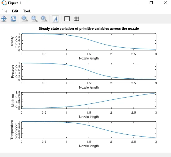
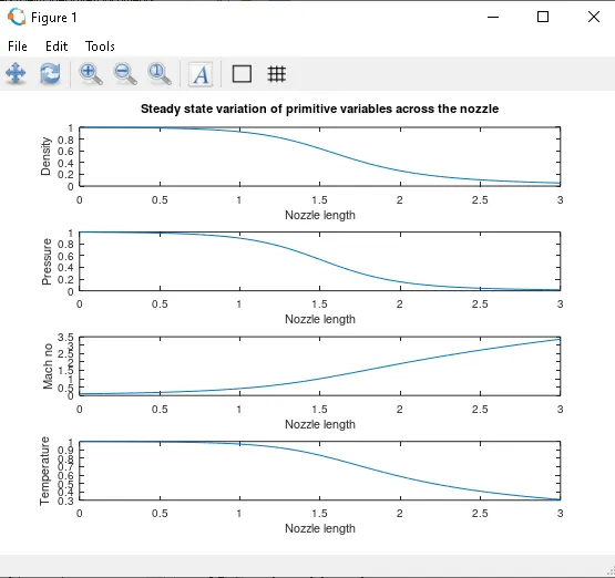
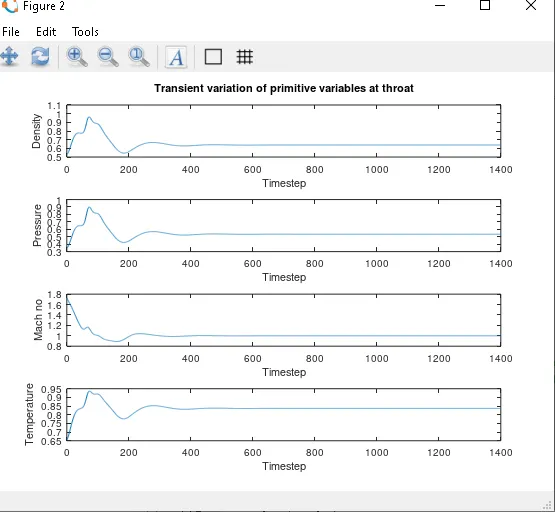
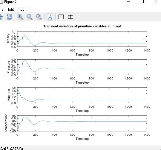
For N = 31 N = 61
Non-conservative form:-
Conservative form:-
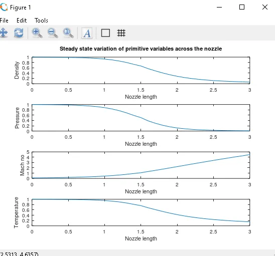
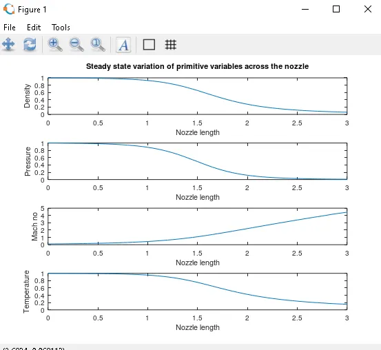
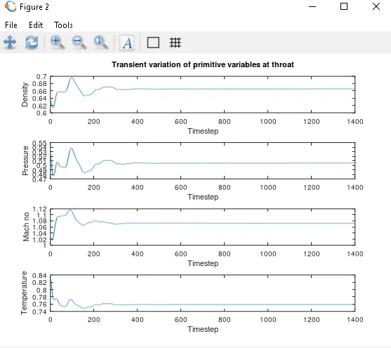
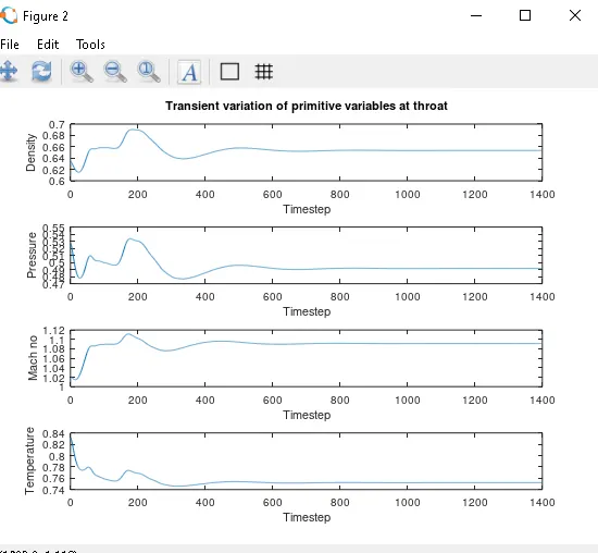
From the above graphs we can conclude that the initial variation in non-conservative forms for a certain period of time makes it consumes higher amount of time to achieve stable solution when comapred to conserved form.
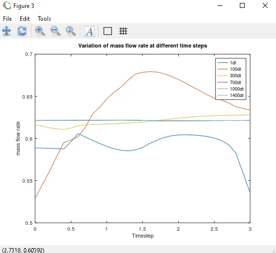
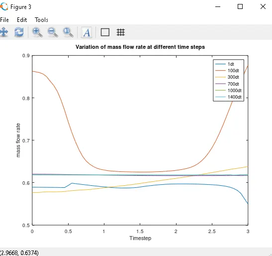
Variation of mass flow distribution through the nozzle at different times during the time-marching process, solution of the conservation form of the governing equations.From the above plots of variation in mass flow rate at different time steps at N = 31 grid points the mass is conserved after the 1400 steps whereas in the N = 61 the mass is conserved after the 700 time steps.
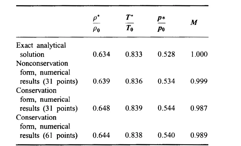
Comparison between the conservative and Non-conservative form:The above discussion does not necessarily establish a definite superiority of the conservation form results over the nonconservation form results. Quite the contrary, let us take a look at the primitive variables; in particular, temperature, pressure, and Mach number at the nozzle throat.The first row gives the exact, analytical results. The second and third rows give the numerical results for the nonconservation and the conservation forms, respectively.
Note that the nonconservation form results are distinctly closer to the exact
values. The last row gives conservation form results for a grid with twice as many grid points (61 in comparison to 31 points). A comparison of the last two rows are an indication of grid independence for the conservation form results. Note that, by doubling the number of grid points, the steady-state numerical results are slightly closer to the exact, analytical values (but still not as close as the nonconservation form results with half as many grid points). For all practical purposes, we have grid independence with 31 grid points.
The behavior of the residuals for the conservation form is not as good as that for the nonconservation form of the equations. For the nonconservation form, that at early times the residuals are on the order of 10-1, but they decay to about IO - 6 after 1400 time steps. In contrast, for the conservation form of the equations, the residuals at early times are on the order of I 0-1 but decay only to about 10-3 after 1400 time steps. However, this is sufficient to produce the steadystate results, for all practical purposes.for the given flow problem, we cannot establish a clear superiority of the conservation form of the governing equations over the nonconservation form.
1.The conservation form yields a better mass flow distribution. The conservation form simply does a better job of conserving mass.
2. The nonconservation form leads to smaller residuals. The amount by which the residuals decay is often used as an index of "quality" of the numerical algorithm. In this sense, the non-conservation form does a better job.
3. There is no clear superiority of either form in terms of accuracy of the results. The nonconservation form seems to produce slightly more accurate results for the primitive variables, and the conservation form seems to produce slightly more accurate results for the flux variables. The results in either case are certainly satisfactory.
4.Most of this is due to the need to decode the primitive variables from the flux variables; such decoding is not necessary when you are solving the nonconservation form.