Week 7 - Simulation of a 1D Super-sonic nozzle flow simulation using Macormack Method
MACORMACK METHOD
AIM: To write program for simulating 1D super-sonic flow nozzle using McCormack method.
OBJECTIVES:
- Steady-state distribution of primitive variables inside the nozzle.
- Time-wise distribution of the primitive variables
- Variation of the mass flow rate distribution inside the nozzle at different time steps during the time marching process.
- Comparison of normalized mass flow rate distributions of both forms.
THEORY:
Convergent-Divergent Nozzle:
This nozzle is used to obtain a supersonic stream starting from low speeds at the inlet .Then the Mach number should increase from Ma=0 near the inlet to Ma>1 at the exit. It is clear that the nozzle must converge in the subsonic portion and diverge in the supersonic portion. Such a nozzle is called a convergent-divergent nozzle. A convergent-divergent nozzle is also called a de laval nozzle.
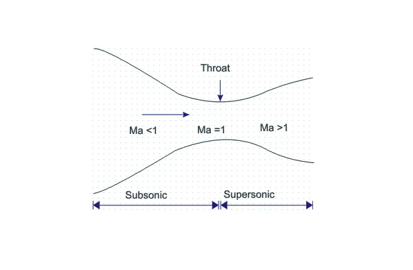
We consider the study isentropic flow through a convergent divergent nozzle sketched below. The flow at the inlet to the nozzle comes from a reservoir where the pressure and temperature are denoted by `P_o` and `T_o` respectively. The cross-sectional area of the reservoir is large and hence the velocity is very small. Thus Po and To are the stagnation values, or total pressure and total temperature, respectively. The flow expands isentropically to supersonic speeds at the nozzle exit where the exit pressure, temperature, velocity and Mach number are denoted by `P_e,T_e,V_e,M_e` respectively. The flow is locally subsonic in the convergent section of the nozzle, sonic at the throat and supersonic at the divergent section. The sonic flow at the throat means that the local velocity at this location is equal to local speed of sound. Using an * to denote sonic flow values we have at the throat. Similarly the sonic flow values of pressure and temperature are denoted by`P^(ast)` and `T^(ast)` respectively. The area of the sonic throat is denoted by `A^(ast)`. We assume that at a given section where the cross sectional area is A, flow properties are uniform across that section. Hence, although the area of nozzle changes as a function of distance along the nozzle, `x`, and therefore in reality e the flow is two dimensional, we make the assumption that the flow properties vary only with `x`. Such flow is defined as quasi one dimensional flow.
GOVERNING EQUATIONS:
Non-Conservative form:
Continuity Equation
`(delrho^')/(delt^')=-rho'(delV')/(delx')-rho'V'(del(lnA'))/(delx')-V'(delrho')/(dx')`
Momentum Equation
`(delV')/(delt')=-V'(delV')/(delx')-1/(gamma)((delT')/(delx')+(T')/(rho')(delrho')/(delx'))`
Energy Equation
`(delT')/(delt')=-V'(delT')/(delx')-(gamma-1)T'[(delV')/(delx')+V'(dellnA')/(delx')]`
Conservative Form:
Continuity Equation
`(del(rho'A'))/(delt')+(del(rho'A'V'))/(delx')=0`
Momentum Equation
`(del(rho'A'V'))/(delt')+(del[(rho'A'(V')^2+(1/gamma)p'A')])/(delx')=(1/gamma)p'(delA')/(delx')`
Energy Equation
`(del[rho'((e')/(gamma-1)+gamma/2(V')^2)A'])/(delt')+(del[rho'((e')/(gamma-1)+gamma/2(V')^2)V'A'+p'A'V'])/(delx')=0`
Finite Difference Equations:
To implement a finite difference solution, we divide x axis along the nozzle into number of discrete grid points.
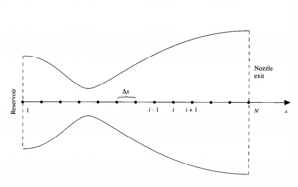
The first point of grid labeled as 1, is referred a reservoir .The points are evenly distributed the along x axis with dx denoting the space between the grid points. The last point of the grid namely the nozzle exit is denoted by N. Point ‘i’ is simply an arbitrary grid point with points i+1 and i-1 as the adjacent points. McCormack method is predictor-corrector method. In time marching solution we now the values of properties at time step t and we use them to find the property values at time step t+dt using explicit scheme.
Non-conservative form:
In Predictor step we use forward differencing for spacial derivatives.
Continuity Equation:

Momentum Equation:

Energy Equation:

By using the above derivative we can get the perdicted values of rho,v and T
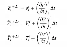
Now we use correcter step, where we use the values of properties at time step t+dt. In corrector step we do backward differencing for spacial derivatives.
Continuity Equation:
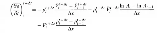
Momentum Equation:

Energy Equation:
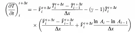
By using the above equations we get the average time derivatives
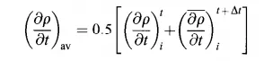
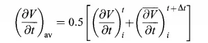
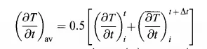
We subsitiute the values of above equations in below given forms to find the second order accuarte values of rho, V and T
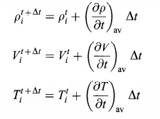
Conservation form:
The equations for quasi-one-dimensional flow can be expressed in generic form . Let us define the elements of solutions vector U, the flux vector F and the source term L as follows
`U_1'=rho'A'`
`U_2=rho'A'V'`
`U_3=rho'((e')/(gamma-1)+gamma/2(V')^2)A'`
`F_1=rho'A'V'`
`F_2=rho'A'(V')^2+(1/gamma)p'A'`
`F_3=rho'((e')/(gamma-1)+gamma/2(V')^2)V'A'+p'A'V'`
`L_2=(1/gamma)p'(delA')/(delx')`
First we will find the source vectors with the above equations with initial conditions, and then we can find the flux vectors.
`F_1=U_2`
`F_2=U_2^2/(U_1)+(gamma-1)/(gamma)(U_3-gamma/2U_2^2/(U_1))`
`F_3=gamma(U_2U_3)/U_1-(gamma(gamma-1))/2U_2^3/U_1^2`
`L_2=(gamma-1)/gamma(U_3-gamma/2U_2^2/U_1)(del(lnA'))/(delx')`
Predictor Step :
Then we set up the spatial derivatives as forward differences
`((dU_1)/(dt'))^(t')=-((F_1)_(i+1)-(F_1)_i)/(Deltax')`
`((dU_2)/(dt'))^(t')=-((F_2)_(i+1)-(F_2)_i)/(Deltax')+L_2`
`((dU_3)/(dt'))^(t')=-((F_3)_(i+1)-(F_3)_i)/(Deltax')`
Then we find the predicted values of U1, U2 and U3
`(U_1)^(t'+Deltat')=(U_1)^(t')+((delU_1)/(delt'))^(t')(Deltat')`
`(U_2)^(t'+Deltat')=(U_2)^(t')+((delU_2)/(delt'))^(t')(Deltat')`
`(U_3)^(t'+Deltat')=(U_3)^(t')+((delU_3)/(delt'))^(t')(Deltat')`
Using these values we will find the predicted values of the primitive variables
`(rho')^(t'+Deltat')=(U_1)^(t'+Deltat')/(A')`
`(T')^(t'+Deltat')=(gamma-1)[(U_3)^(t'+Deltat')/(U_1)^(t'+Deltat')-gamma/2((U_2)^(t'+Deltat')/((U_1)^(t'+Deltat')))^2]`
Now update the flux vectors with new density ,velocity and temperature
Corrector Step:
We have the predicted values of the flow properties. In corrector step we use the backward differencing for the spacial derivatives.
`((dU_1)/(dt'))^(t'+Deltat')=-((F_1)_(i)-(F_1)_(i-1))/(Deltax')`
`((dU_2)/(dt'))^(t'+Deltat')=-((F_2)_(i)-(F_2)_(i-1))/(Deltax')+L_2`
`((dU_3)/(dt'))^(t'+Deltat')=-((F_3)_(i)-(F_3)_(i-1))/(Deltax')`
From the above equations we get the average derivative values
`((delU_1)/(delt'))_(avg)=1/2[((delU_1)/(delt'))^(t')+((delU_1)/(delt'))^(t'+Deltat')]`
`((delU_2)/(delt'))_(avg)=1/2[((delU_2)/(delt'))^(t')+((delU_2)/(delt'))^(t'+Deltat')]`
`((delU_3)/(delt'))_(avg)=1/2[((delU_3)/(delt'))^(t')+((delU_3)/(delt'))^(t'+Deltat')]`
The corrected values of U1,U2,U3 are
`(U_1)^(t'+Deltat')=(U_1)^(t')+((delU_1)/(delt'))_(avg)(Deltat')`
`(U_2)^(t'+Deltat')=(U_2)^(t')+((delU_2)/(delt'))_(avg)(Deltat')`
`(U_3)^(t'+Deltat')=(U_3)^(t')+((delU_3)/(delt'))_(avg)(Deltat')`
Now from the above equations we can find the final primitive variables
`(rho')^(t'+Deltat')=(U_1)^(t'+Deltat')/(A')`
`(V')^(t'+Deltat')=(U_2)^(t'+Deltat')/((U_1)^(t'+Deltat')`
`(T')^(t'+Deltat')=(gamma-1)[(U_3)^(t'+Deltat')/(U_1)^(t'+Deltat')-gamma/2((U_2)^(t'+Deltat')/((U_1)^(t'+Deltat')))^2]`
Courant Number :
Time step can be calculated by using Courant number
`Deltat=C(Deltax)/(a+V)`
Where
C= courant number
`Deltax`= spacial difference
`Deltat`= Time step
`a`= Velocity of sound
`V`=velocity of the object
Will use this equation at each grid point and calculate the time step value at each grid point. Now find the minimum timestep value among all those grids and use that as time step for calculation.
MAIN PROGRAM:
% Simulation of Convergent-Divergent Nozzle using McCormack Method

clear all
close all
clc

%Inputs

% number of grids points
n=31;

% x-cordinate values
x=linspace(0,3,n);

%spacial difference
dx=x(2)-x(1);

% Total number of timsteps
nt=1400;

% Calling the Non-conservative function
[rho,v,t,P,M,rho_t,v_t,t_t,P_t,M_t,mass]=non_conservative(x,n,dx,nt);

% Calling the Conservative function
[rho_c,v_c,t_c,P_c,M_c,rho_tc,v_tc,t_tc,P_tc,M_tc,mass_c]=conservative(x,n,dx,nt);

% Properties of the Non-conservative form
figure(1)

% Plotting mach number
subplot(4,1,1)
plot(x,M);
title('steady state variation of primitive variables - Non Conservation form');
xlabel('Distance');
ylabel('Mach Number');

%Plotting Pressure
subplot(4,1,2)
plot(x,P);
xlabel('Distance');
ylabel('Pressure');

%Plotting Temperature
subplot(4,1,3)
plot(x,t);
xlabel('Distance');
ylabel('Temperature');

%Plotting density
subplot(4,1,4)
plot(x,rho);
xlabel('Distance');
ylabel('Density');

%Non-Conservative Form variation of properties at throat
figure(2)

% Plotting density at throat
subplot(4,1,1)
plot(1:1400,rho_t);
title('Transient variation of primitive variables at throat - Non Conservation form');
xlabel('No.of timesteps');
ylabel('Density');

%Plotting Mach at throat
subplot(4,1,2)
plot(1:1400,M_t);
xlabel('No.of time steps ');
ylabel('Mach Number');

%Plotting Pressure at throat
subplot(4,1,3)
plot(1:1400,P_t);
xlabel('No.of time steps ');
ylabel('Pressure');

% Plotting temperature at throat
subplot(4,1,4)
plot(1:1400,t_t);
xlabel('No.of timesteps ');
ylabel('Temperature');


% Properties of Conservative form
figure(3)
subplot(4,1,1)

%Plotting mach
plot(x,M_c);
title('steady state variation of primitive variables - Conservation form');
xlabel('Distance');
ylabel('Mach Number');

%Plotting pressure
subplot(4,1,2)
plot(x,P_c);
xlabel('Distance');
ylabel('Pressure');

%Plotting Tempearture
subplot(4,1,3)
plot(x,t_c);
xlabel('Distance');
ylabel('Temperature');

%Plotting density
subplot(4,1,4)
plot(x,rho_c);
xlabel('Distance');
ylabel('Density');


%Conservative Form variation of properties at throat
figure(4)

%Plotting density
subplot(4,1,1)
plot(1:1400,rho_tc);
title('Transient variation of primitive variables at throat - Conservation form');
xlabel('No.of timesteps');
ylabel('Density');

%Plotting Mach number
subplot(4,1,2)
plot(1:1400,M_tc);
xlabel('No.of time steps ');
ylabel('Mach Number');

%plotting pressure
subplot(4,1,3)
plot(1:1400,P_tc);
xlabel('No.of time steps ');
ylabel('Pressure');

%Plotting temperature
subplot(4,1,4)
plot(1:1400,t_t);
xlabel('No.of timesteps ');
ylabel('Temperature');


%Steady state Mass flow rate comparison
figure(5)

% plotting the mas flow rate of non-conservative form
plot(x,mass)
hold on;
%Plotting the mass flow arte of conservative form
plot(x,mass_c)
xlabel('Length of Nozzle');
ylabel('Flow rate');
legend('Non-Conservation form','Conservation form');
Function for Non-conservative form:
%Non-Conservative function

function [rho,v,t,P,M,rho_t,v_t,t_t,P_t,M_t,mass]=non_conservative(x,n,dx,nt)

% Density profile
rho=1-0.346*x;

%Temperature profile
t=1-0.2314*x;

%Velocity profile
v=(0.1+1.09*x).*t.^(1/2);

%Area profile
a=1+(2.2*(x-1.5).^2);

% specific ratio
gamma=1.4;

%time step
delta_t=0.5*(dx./((sqrt(t)+v)));
dt=min(delta_t);

% Throat loaction
throat=find(a==1);

%time marching
for k=1:nt

    %assiging the inital values to old variables
    rho_old=rho;
    v_old=v;
    t_old=t;

    %predictor Method
    for i=2:n-1
        dvdx=(v(i+1)-v(i))/dx;
        drhodx=(rho(i+1)-rho(i))/dx;
        dtdx=(t(i+1)-t(i))/dx;
        dlogadx=(log(a(i+1))-log(a(i)))/dx;

        %Continity equation
        drhodt_p(i)=-rho(i)*dvdx-rho(i)*v(i)*dlogadx-v(i)*drhodx;
        %Momentum equation
        dvdt_p(i)=-v(i)*dvdx-(1/gamma)*(dtdx+(t(i)/rho(i))*drhodx);
        %Energy equation
        dtdt_p(i)=-v(i)*dtdx-(gamma-1)*t(i)*(dvdx+v(i)*dlogadx);

    end

   %Solution Update
   for i=2:n-1
    rho(i)=rho(i)+drhodt_p(i)*dt;
    v(i)=v(i)+dvdt_p(i)*dt;
    t(i)=t(i)+dtdt_p(i)*dt;
   end

    %Corrector method
         for j=2:n-1
        dvdx=(v(j)-v(j-1))/dx;
        drhodx=(rho(j)-rho(j-1))/dx;
        dtdx=(t(j)-t(j-1))/dx;
        dlogadx=(log(a(j))-log(a(j-1)))/dx;

        %Continity equation
        drhodt_c(j)=-rho(j)*dvdx-rho(j)*v(j)*dlogadx-v(j)*drhodx;
        %Momentum equation
        dvdt_c(j)=-v(j)*dvdx-(1/gamma)*(dtdx+(t(j)/rho(j))*drhodx);
        %Energy equation
        dtdt_c(j)=-v(j)*dtdx-(gamma-1)*t(j)*(dvdx+v(j)*dlogadx);

     end

     %Average time derivatives
     rho_avg=0.5*(drhodt_p+drhodt_c);
     v_avg=0.5*(dvdt_p+dvdt_c);
     t_avg=0.5*(dtdt_p+dtdt_c);

     %Solution update
          for m=2:n-1
         rho(m)=rho_old(m)+rho_avg(m)*dt;
         v(m)=v_old(m)+v_avg(m)*dt;
         t(m)=t_old(m)+t_avg(m)*dt;
          end

     %inlet boundary condition
     v(1)=2*v(2)-v(3);

     %outlet boundary conditions
     v(n)=2*v(n-1)-v(n-2);
     rho(n)=2*rho(n-1)-rho(n-2);
     t(n)=2*t(n-1)-t(n-2);

     %Mach number
     M=(v./sqrt(t));

     %Pressure
     P=rho.*t;

     %flow Property values at throat

     rho_t(k)=rho(throat);
     t_t(k)=t(throat);
     v_t(k)=v(throat);
     P_t(k)=P(throat);
     M_t(k)=M(throat);

     %mass flow rate
     mass=rho.*v.*a;

     %plot the variation of mass flow rate throught the process
      figure (6)

     % At timestep 50
     if k==50
         plot(x,mass,'linewidth',2)
         hold on;

         % At timestep 100
    elseif k==100
         plot(x,mass,'linewidth',2)

         % At timestep 200
    elseif k==200
        plot(x,mass,'linewidth',2)

         % At time step 400
    elseif k==400
         plot(x,mass,'linewidth',2)

       % At time step 600
     elseif k==600
         plot(x,mass,'linewidth',2)

    % At time step 800
    elseif k==800
         plot(x,mass,'linewidth',1)
         title('Plot of mass flow rates at different time steps(non-conservative)');
         xlabel('distance');
         ylabel('Non-dimensional mass flow rate');
         legend('50','200','400','600','800');
     end
end
end
Function for Conservative form:
%Conservative Form

function[rho_c,v_c,t_c,P_c,M_c,rho_tc,v_tc,t_tc,P_tc,M_tc,mass_c]=conservative(x,n,dx,nt)


% Profile variations of density and tempearture wrt to value of x

%when the value of x is btw 1.5 and 3
for i=1:length(x)

    if (x(i)>=1.5 &&x(i)<=3)

       rho(i)=0.634-0.3879*(x(i)-1.5);
       t(i)=0.833-0.3507*(x(i)-1.5);
    end
end

%when the value of x is btw 0.5 and 1.5
for i=1:length(x)
    if (x(i)>=0.5 && x(i)<=1.5)

       rho(i)=1-0.366*(x(i)-0.5);
       t(i)=1-0.167*(x(i)-0.5);
    end
end

%when the value of x is btw 0 and 0.5
for i=1:length(x)
    if (x(i)>=0 && x(i)<=0.5)

       rho(i)=1;
       t(i)=1;
    end
end

% Area profile btw 0 and 3
a=1+(2.2*(x-1.5).^2);

% Velocity profile
v=(0.59)./(rho.*a);

% Specific ratio
gamma=1.4;

%time step
delta_t=0.5*(dx./((sqrt(t)+v)));
dt=min(delta_t);

%Solution vector
U1=rho.*a;
U2=U1.*v;
U3=rho.*((t./(gamma-1))+(gamma/2).*v.^2).*a;

for k=1:nt
    U1_old=U1;
    U2_old=U2;
    U3_old=U3;

    %Flux vector
    F1=U2;
    F2=((U2.^2)./U1)+((gamma-1)/gamma)*(U3-(gamma/2)*(((U2).^2)./U1));
    F3=(((gamma)*(U2.*U3))./U1)-(((gamma*(gamma-1)/2)*(((U2).^3)./(U1).^2)));

    %Predictor step
    for j=2:n-1

        L2(j)=(1/gamma)*rho(j)*t(j)*((a(j+1)-a(j))/dx);
        dU1dt_p(j)=-((F1(j+1)-F1(j))/dx);
        dU2dt_p(j)=-((F2(j+1)-F2(j))/dx)+L2(j);
        dU3dt_p(j)=-((F3(j+1)-F3(j))/dx);

        %Solution update

        U1(j)=U1_old(j)+(dU1dt_p(j))*dt;
        U2(j)=U2_old(j)+(dU2dt_p(j))*dt;
        U3(j)=U3_old(j)+(dU3dt_p(j))*dt;

    end

    %Solution
    rho=(U1./a);
    v=(U2./U1);
    t=(gamma-1)*((U3./U1)-(gamma/2)*(v).^2);

    %Updating the flux vector

    F1=U2;
    F2=((U2.^2)./U1)+((gamma-1)/gamma)*(U3-(gamma/2)*(((U2).^2)./U1));
    F3=(((gamma)*(U2.*U3))./U1)-(((gamma*(gamma-1)/2)*(((U2).^3)./(U1).^2)));

    %Corrector step
    for m=2:n-1

        L2(m)=(1/gamma)*rho(m)*t(m)*((a(m)-a(m-1))/dx);
        dU1dt_c(m)=-((F1(m)-F1(m-1))/dx);
        dU2dt_c(m)=-((F2(m)-F2(m-1))/dx)+L2(m);
        dU3dt_c(m)=-((F3(m)-F3(m-1))/dx);

    end

    %Average time deravative

    dU1dt_avg = 0.5*(dU1dt_p+dU1dt_c);
    dU2dt_avg = 0.5*(dU2dt_p+dU2dt_c);
    dU3dt_avg = 0.5*(dU3dt_p+dU3dt_c);

    % Update of final values
    for i=2:n-1
        U1(i)=U1_old(i)+dU1dt_avg(i)*dt;
        U2(i)=U2_old(i)+dU2dt_avg(i)*dt;
        U3(i)=U3_old(i)+dU3dt_avg(i)*dt;

    end

    %Solution Update
    rho_c= U1./a;
    v_c=(U2./U1);
    t_c=(gamma-1)*((U3./U1)-(gamma/2)*(v_c).^2);

    %defining inlet flow boundary conditions
    U1(1)=rho_c(1)*a(1);
    U2(1)=2*U2(2)-U2(3);
    v_c(1)=U2(1)/U1(1);
    U3(1)=U1(1)*(t(1)/(gamma-1)+(gamma/2)*v_c(1)^2);

    %Outflow boundary conditions
    U1(n)=2*U1(n-1)-U1(n-2);
    U2(n)=2*U2(n-1)-U2(n-2);
    U3(n)=2*U3(n-1)-U3(n-2);

    % Mach number
     M_c=(v_c./sqrt(t));

     % Pressure
     P_c=rho_c.*t_c;

     %throat position
     throat=find(a==1);

     %Values of density, Tempearture, pressure,Mach and velocity at throat
     rho_tc(k)=rho_c(throat);
     t_tc(k)=t_c(throat);
     v_tc(k)=v_c(throat);
     P_tc(k)=P_c(throat);
     M_tc(k)=M_c(throat);

     %Mass flow rate
     mass_c= rho_c.*a.*v_c;

     % Plotting the variation of mass flow rate in conservative approach at
     % different time steps

     figure(7)
      if k==50
         plot(x,mass_c,'linewidth',2)
         hold on;

    elseif k==100
         plot(x,mass_c,'linewidth',2)

   elseif k==200
         plot(x,mass_c,'linewidth',2)

   elseif k==400
        plot(x,mass_c,'linewidth',2)

     elseif k==600
         plot(x,mass_c,'linewidth',2)

   elseif k==800
         plot(x,mass_c,'linewidth',1)
         title('Plot of mass flow rates at different time steps(conservative)');
         xlabel('distance');
         ylabel('Non-dimensional mass flow rate');
         legend('50','200','400','600','800');


      end
end

end
EXPLANANTION OF CODE:
1. Clear all command is used to clear all the data in workspace.
2. close all command is used to clear all the figures
3. clc is used to clear the command window
4. Input values are given and the functions for conservative and non-conservative are written.
5. flow property profiles are defined and late by using governing equations of both the forms, the derivative values at time step 't' are calculated.
6. This done by using McCormack method , in which we use predictor -corrector form.
7. After calculating the finals plot are made wrt to x values and wrt to the number of timsteps
8. Title, labelling and legends are given for all the plots using respective commands
OUTPUTS :
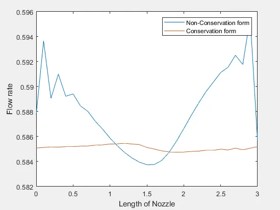
Plot for massflow rate comparsion:
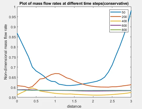
Plot for mass flow rate at different time steps(Conservative ):
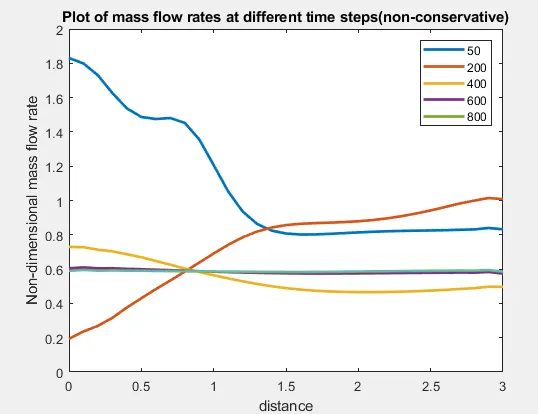
Plot for mass flow rate at different time steps(Conservative ):
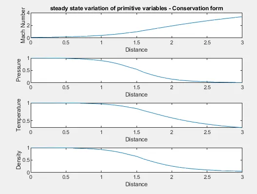
Plot for steady state variation of primitive variables(Conservative):
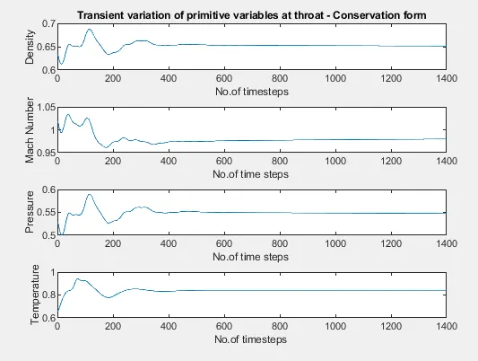
Plot for transient variation of primitive variables(Conservative):
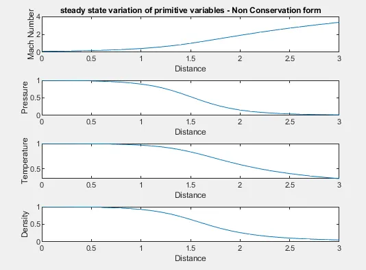
lot for steady state variation of primitive variables(Non-Conservative):
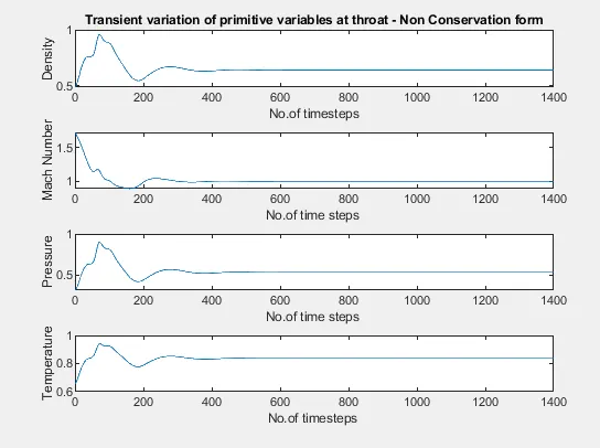
Plot for transient variation of primitive variables(Non-Conservative):
Grid Independence test:
For n=31 For n=61
Flow variables at throat Anaylytical Cons Non-Cons Cons Non-cons
Density 0.634 0.6515 0.6387 0.6389 0.6377
Pressure 0.528 0.5476 0.5342 0.5337 0.5327
Mach number 1 0.9797 0.9994 0.9982 0.9998
Temperature 0.833 0.8406 0.8365 0.8354 0.8354
Above given values for density,Temperature, Mach and Pressure at throat in Conservative, Non-conservative and analytical forms.From the above we can observe that the Values of the conservative and Non-conservative are almost equal .However, non-conservative form is more accuarate when compared to conservative form.We can also observe that the values of conservative form are most accurate when no.of grids are 61 , wheras 31 grid points is the case with non-conservative form . It can also be said that the conservative form is grid independent at n=61 and non-conservative form is grid independent at n=31.
CONCLUSIONS:
1. From the above we can conclude that conservative form yeilds a better mass flow rate distribution as it maintains almost constant graph throught which is not the case with non-conservative form.In non-conservative form the graph is distracted more at the inlet and outlet.
2. From the mass flow rate graph with resepct to time we can observe that around 700-800 time steps mass flow rate reached steady state both in conservative and non-consevative forms.
3. From the above graphs we can that Mach number is less than 1 at inlet as it a subsonic zone later that got increased to 1 at throat and final to greater than 1 at the end of nozzle. A Mach increases velocity of the obejct increases , which inturn concludes at as velcoity increases pressure and density decreases. From gas equation we can also say that as pressure decreases density alos decreases across the flow.
4.Non-conservative form is easy to program beacuse they are solved interm of primitive varaible whereas we used flux varaible source terms in conservative form, which makes process difficult. Apart from that utilization of more terms results in increase in error percentage . So interms of accuracy also non-conservative form is preferred to conservative form.
5. In non-conservative form the residual decays are faster comapred to conservative form,which can been assesed from the values obtained in grid independence test. The amount of residual decay is often used to judge the quality of numerical alogorthim. so non-conservative form is better.