Week 7 - Simulation of a 1D Super-sonic nozzle flow simulation using Macormack Method
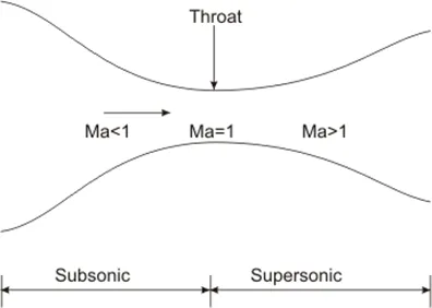
Subsonic Supersonic Isentropic flow thorough convergent divergent nozzle.
- Consider the steady ,isentropic flow through convergent divergent nozzle as shown in the figure.
- The flow enters in the nozzle from the reservoir where the pressure and temperature is denoted by p0 and T0
- The cross sectional area is assumed to be very large so the velocity at the inlet is going to be nearly equal to zero.
- Thus the p0 and T0 are the staganation values or the total pressure and the total temperature .
- The flow expands isentropically to supersonic speeds and the values at the exit are pe ,Te, ve Me
- We assume that the flow propertities are uniform across any cross section of the nozzle, that means that the flow propertities are function of x only this type of the flow is called the quasi one dimensional flow.
Non conservative form of governing equation
Continuity equation
`(delrho')/(delt')=-rho'*(delv')/(delx')-rho'*v'*(dellogA')/(delx')-v'*(delrho')/(delx')`
Momentum equation
`(delv')/(delt')=-v'*(delv')/(delx')-1/gamma*((delT')/(delx')+(T')/(rho')*(delrho')/(delx'))`
Energy equation
`(delT')/(delt')=-v'*(delT')/(delx')-(gamma-1)*T'*((delv')/(delx')+v'*(dellogA')/(delx'))`
Conservative form of governing equation
continuity equation
`(delrho'A')/(delt')+(delrho'A'v')/(delx')=0`
momentum equation
`(delrho'A'V')/(delt')+(del(rho'A'v'^2+(1/gamma)p'A'))/(delx')=(1/gamma)*p'*(delA')/(delx')`
energy equation
`(del(rho'(e'/(gamma-1)+gamma/2*v'^2)*A'))/(delt')+(del(rho'(e'/(gamma-1)+gamma/2*v'^2)*A'*v'+p'A'v'))/(delx')=0`
here we are using the mecormack method to solve the governing equation numerically
1)first we have to specify the values of temperature,density and velocity which are the assumed values.
2)now let the function for the solving the temperature density and velocity is f(x),so first we have to perform the predictor step.
`((delf)/(delt)) =(f(i+1)-f(i))/(Delta(x))`
3)update the solution after the predictor step
`fundersetp=funderset("initial")+((delf)/(delt))undersetp *Deltat`
4)corrector step
`((delf)/(delt))undersetc =(f(i)-f(i-1))/(Delta(x))`
5)finding the avg of the predictor and corrector step
`(delf)/(delt)avg=(delf)/(delt)p+(delf)/(delt)c`
6)final solution update
`fsol=f(nitial)+(delf)/(delt)avg*Deltat`
main code
clear all
close all
clc

%inputs
L=3;   %length of the nozzle

n=[31];
nt=1400;
for i=1:length(n)

[mfr]=conservative_nozzle(L,n(i),nt)
[mfr]=non_conservative(L,n(i),nt)
end
Matlab function for the conservative method
function [mfr]=conservative_nozzle(L,n,nt)
C=0.5;     %cfl number
x=linspace(0,L,n)
dx=x(2)-x(1)
gamma=1.4;


%% calculate the initial conditions
for i=1:n
if (x(i)>=0 && x(i)<0.5)
    rho(i)=1;
    T(i)=1;
elseif (x(i)>=0.5 && x(i)<=1.5)
    rho(i)=1-0.366.*(x(i)-0.5);
    T(i)=1-0.167.*(x(i)-0.5);
elseif (x(i)>=1.5 && x(i)<=3.5)
    rho(i)=0.634-0.3879.*(x(i)-1.5);
    T(i)=0.833-0.3507.*(x(i)-1.5);
end
end
A=1+2.2*(x-1.5).^2;
v=0.59./(rho.*A);

% defining the solution vector
U1=rho.*A;
U2=rho.*A.*v;
U3=rho.*A.*(T./(gamma-1)+(gamma/2).*v.^2);

%calculation of the time steps
dt=min(C*(dx./(T.^0.5+v)));
%% predictior step
for k=1:nt

    % retaining the old copy of the solution vector
    U1_old=U1;
    U2_old=U2;
    U3_old=U3;


    % updating the flux terms
        F1=U2;
        F2=(U2.^2./U1)+((gamma-1)/gamma)*(U3-(gamma/2)*(U2.^2./U1));
        F3=(gamma*((U2.*U3)./U1)) - (gamma*(gamma-1)/2)*(U2.^3./U1.^2);

    for j=2:n-1

        J2(j)=(1/gamma)*rho(j)*T(j)*((A(j+1)-A(j))/dx);

        %continuity equation
        dU1dt_p(j)=-(F1(j+1)-F1(j))/dx;

        % momentum equation
        dU2dt_p(j)=-((F2(j+1)-F2(j))/dx)+J2(j);

        % energy equation
        dU3dt_p(j)=-(F3(j+1)-F3(j))/dx;

        %solution update
        U1(j)=U1_old(j)+dU1dt_p(j)*dt;
        U2(j)=U2_old(j)+dU2dt_p(j)*dt;
        U3(j)=U3_old(j)+dU3dt_p(j)*dt;
    end
    % updating the flux terms
        F1=U2;
        F2=(U2.^2./U1)+((gamma-1)/gamma)*(U3-(gamma/2)*(U2.^2./U1));
        F3=(gamma*((U2.*U3)./U1)) - (gamma*(gamma-1)/2)*(U2.^3./U1.^2);


        % updating the rho and T for the J value in corrector step

        rho=U1./A
        T=(gamma-1)*((U3./U1)-(gamma/2)*(U2./U1).^2);


        for j=2:n-1

    J2(j) = (1/gamma)*rho(j)*T(j)*(A(j)-A(j-1))/dx;

    %Corrected method
    %continuity equation:
    dU1dt_c(j)=-(F1(j)-F1(j-1))/dx;

    %Momentum equation:
    dU2dt_c(j)=-((F2(j)-F2(j-1))/dx)+J2(j);

    %Energy equation:
    dU3dt_c(j)=-(F3(j)-F3(j-1))/dx;
       end

    % finding the avg

    dU1_dt_avg=(dU1dt_p+dU1dt_c)*0.5;
    dU2_dt_avg=(dU2dt_p+dU2dt_c)*0.5;
    dU3_dt_avg=(dU3dt_p+dU3dt_c)*0.5;

    % final values update

    for r=2:n-1

        U1(r)=U1_old(r)+dU1_dt_avg(r)*dt;
        U2(r)=U2_old(r)+dU2_dt_avg(r)*dt;
        U3(r)=U3_old(r)+dU3_dt_avg(r)*dt;
    end

    %initial  condition
    U1(1)=A(1);
    U2(1)=2*U2(2)-U2(3);
    U3(1)=U1(1)*(T(1)/(gamma-1)+(gamma*(U2(1)/U1(1))^2)/2);

    % exit boundary condition

    U1(n)=2*U1(n-1)-U1(n-2);
    U2(n)=2*U2(n-1)-U2(n-2);
    U3(n)=2*U3(n-1)-U3(n-2);

    %  final update of primitives

    rho=U1./A;
    v=U2./U1;
    T=(gamma-1).*(U3./U1-(gamma/2)*(U2./U1).^2);
    p=rho.*T;
    M=v./T.^0.5;
    mfr=rho.*A.*v;


     figure(1)
     subplot(2,3,1)
     plot(x,v)
     xlabel('length of nozzle')
     ylabel('velocity')
     xlim([0 3])
     ylim([0 2])
     text=sprintf('time step=%d',k);
     title(text)
     pause(0.003)

     subplot(2,3,2)
     plot(x,p)
     xlabel('length of nozzle')
     ylabel('pressure')
     xlim([0 3])
     ylim([0 2])
     text=sprintf('time step=%d',k);
     title(text)
     pause(0.003)

     subplot(2,3,3)
     plot(x,rho)
     xlabel('length of nozzle')
     ylabel('density')
     xlim([0 3])
     ylim([0 2])
     text=sprintf('time step=%d',k);
     title(text)
     pause(0.003)

     subplot(2,3,4)
     plot(x,mfr)
     xlabel('length of nozzle')
     ylabel('mass flow rate')
     xlim([0 3])
     ylim([0 2])
     text=sprintf('time step=%d',k);
     title(text)
     pause(0.003)

     subplot(2,3,5)
     plot(x,M)
     xlabel('length of nozzle')
     ylabel('mach number')
     xlim([0 3])
     ylim([0 2])
     text=sprintf('time step=%d',k);
     title(text)
     pause(0.003)


     subplot(2,3,6)
     plot(x,T)
     xlabel('length of nozzle')
     ylabel('Temperature')
     xlim([0 3])
     ylim([0 2])
     text=sprintf('time step=%d',k);
     title(text)
     pause(0.003)
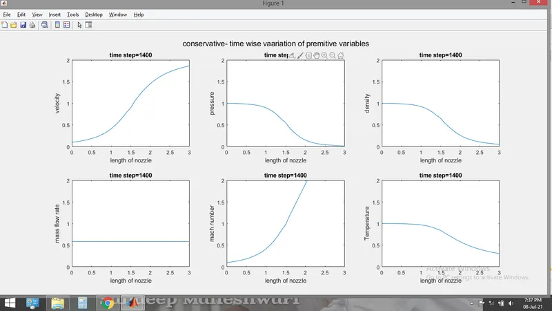
     sgtitle('conservative- time wise vaariation of premitive variables')


end

     figure(2)
     plot(x,v)
     hold on
     plot(x,M)
     hold on
     plot(x,rho)
     hold on
     plot(x,mfr)
     hold on
     plot(x,p)
     hold on
     legend('velocity','mach number','density','mass flow rate','pressure')
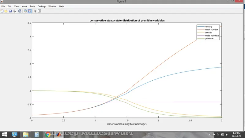
     title(' conservative steady state distribution of premitive variables')
step1)function which takes inputs of n,L and not
step2)giving the inputs of grid points and grid spacing
step3)giving the initial conditions
step4)defining the solution vector
step5)defining the time steps for the various values of dx and taking the minimum value for dt, the courat number is taken as 0.5
step5) defining the for loop for time step
step6)retaining the solution vector old values
step7)defining the flux terms
step8)predictor method for the solution vector by forward differencing
step9)corrector method for the solution vector by backward differencing
step10)calculating the average values
step11)final solution update for the solution vector
step12)calculating the premitive variables from the solution vector
step13)plotting
outputs
Matlab function for the non conservative method
function [mfr]=non_conservative(L,n,nt)

x=linspace(0,3,n);
dx=x(2)-x(1);
gamma=1.4;
%% calculate the initial conditions

rho=1-0.3146*x;
T=1-0.2314*x;
v=(0.1+1.09*x).*T.^0.5;
A=1+2.2*(x-1.5).^2;

%% time steps


C=0.5;     %cfl number
%calculation of the time steps
dt=min(C*(dx./(T.^0.5+v)));

% outer time loop

for k=1:nt


    % predictor method
    rho_old=rho;
    v_old=v;
    T_old=T;

    %continuity equation

    for j=2:n-1

        dvdx=(v(j+1)-v(j))/dx;
        drhodx=(rho(j+1)-rho(j))/dx;
        dTdx=(T(j+1)-T(j))/dx;
        dlogAdx=(log(A(j+1))-(log(A(j))));

        drhodt_p(j)=-rho(j)*dvdx-rho(j)*v(j)*dlogAdx-v(j)*drhodx;


        % momentum equation

        dvdt_p(j)=-v(j)*dvdx-(1/gamma)*(dTdx+(T(j)/rho(j))*drhodx);

        %energy equation

        dTdt_p(j)=-v(j)*dTdx-(gamma-1)*(T(j))*((dvdx)+v(j)*dlogAdx);

        %solution update

        v(j)=v_old(j)+dvdt_p(j)*dt;
        rho(j)=rho_old(j)+drhodt_p(j)*dt;
        T(j)=T_old(j)+dTdt_p(j)*dt;


        %% corrector step


        dvdx=(v(j)-v(j-1))/dx;
        drhodx=(rho(j)-rho(j-1))/dx;
        dTdx=(T(j)-T(j-1))/dx;
        dlogAdx=(log(A(j))-(log(A(j-1))));

        drhodt_c(j)=-rho(j)*dvdx-rho(j)*v(j)*dlogAdx-v(j)*drhodx;


        % momentum equation

        dvdt_c(j)=-v(j)*dvdx-(1/gamma)*(dTdx+(T(j)/rho(j))*drhodx);

        %energy equation

        dTdt_c(j)=-v(j)*dTdx-(gamma-1)*(T(j))*((dvdx)+v(j)*dlogAdx);

    end

    % compute avg time derivative

    drhodt_avg=0.5*(drhodt_p+drhodt_c);
    dvdt_avg=0.5*(dvdt_p+dvdt_c);
    dTdt_avg=0.5*(dTdt_p+dTdt_c);

    %final solution update
    for i=2:n-1

        rho(i)=rho_old(i)+drhodt_avg(i)*dt;
        v(i)=v_old(i)+dvdt_avg(i)*dt;
        T(i)=T_old(i)+dTdt_avg(i)*dt;
    end


    % apply boundary condition
    %inlet
    rho(1)=2*rho(2)-rho(3);
    v(1)=2*v(2)-v(3);
    T(1)=2*T(2)-T(3);
    %outlet

    rho(n)=2*rho(n-1)-rho(n-2);
    v(n)=2*v(n-1)-v(n-2);
    T(n)=2*T(n-1)-T(n-2);

    p=rho.*T;
    M=v./T.^0.5;
    mfr=rho.*A.*v;


  figure(3)
     subplot(2,3,1)
     plot(x,v)
     xlabel('length of nozzle')
     ylabel('velocity')
     xlim([0 3])
     ylim([0 2])
     text=sprintf('time step=%d',k);
     title(text)
     pause(0.003)

     subplot(2,3,2)
     plot(x,p)
     xlabel('length of nozzle')
     ylabel('pressure')
     xlim([0 3])
     ylim([0 2])
     text=sprintf('time step=%d',k);
     title(text)
     pause(0.003)

     subplot(2,3,3)
     plot(x,rho)
     xlabel('length of nozzle')
     ylabel('density')
     xlim([0 3])
     ylim([0 2])
     text=sprintf('time step=%d',k);
     title(text)
     pause(0.003)

     subplot(2,3,4)
     plot(x,mfr)
     xlabel('length of nozzle')
     ylabel('mass flow rate')
     xlim([0 3])
     ylim([0 2])
     text=sprintf('time step=%d',k);
     title(text)
     pause(0.003)

     subplot(2,3,5)
     plot(x,M)
     xlabel('length of nozzle')
     ylabel('mach number')
     xlim([0 3])
     ylim([0 2])
     text=sprintf('time step=%d',k);
     title(text)
     pause(0.003)


     subplot(2,3,6)
     plot(x,T)
     xlabel('length of nozzle')
     ylabel('Temperature')
     xlim([0 3])
     ylim([0 2])
     text=sprintf('time step=%d',k);
     title(text)
     pause(0.003)
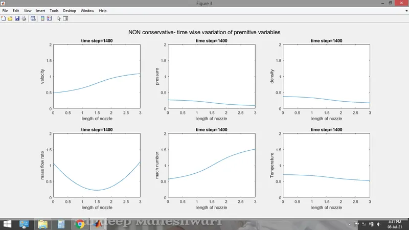
     sgtitle('NON conservative- time wise vaariation of premitive variables')


end

     figure(4)
     plot(x,v)
     hold on
     plot(x,M)
     hold on
     plot(x,rho)
     hold on
     plot(x,mfr)
     hold on
     plot(x,p)
     hold on
     legend('velocity','mach number','density','mass flow rate','pressure')
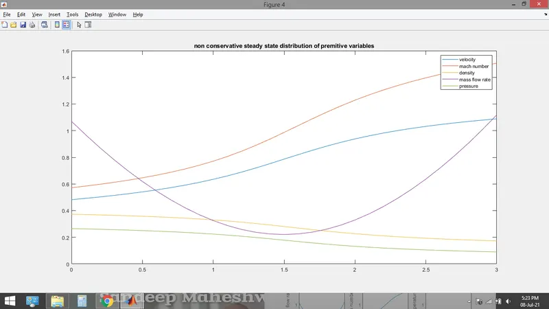
     title('non conservative steady state distribution of premitive variables')
end
step1)function which takes inputs of n,L and not
step2)giving the inputs of grid points and grid spacing
step3)giving the initial conditions
step4)defining the premetive variables
step5)defining the time steps for the various values of dx and taking the minimum value for dt, the courat number is taken as 0.5
step6) defining the for loop for time step
step7)predictor method for the solution vector by forward differencing
step8)corrector method for the solution vector by backward differencing
step9)calculating the average values
step10)final solution update for the premitive variables
step11)plotting